Kriging

Radial basis functions

Implementation in QstatLab

Radial basis functions allow fast approximation of irregular, non-linear functional relationship. The accuracy of the prediction depends on the distance from available data, being exact at an existing data point. Thus its accuracy increases by adding more space filling data. Clusters of data points usually do not improve prediction qualities. The prediction between the data points is controlled using radial basis functions (RBFs).

where

is the Euclidian distance between the data point and the center c. The weights W are computed as a linear solve:

where

and lambda is the regularization factor

There are six RBFs included in QstatLab:

Linear f(r) = r (type = rbf_linear)
Cubic spline f(r) = r^3 (type = rbf_cubic) - default
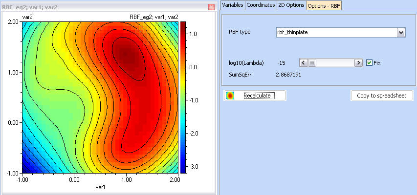
Thin plate spline f(r) = r^2*ln(r) - (type = rbf_thinplate)
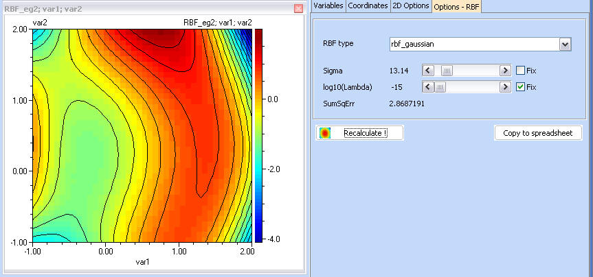
Gaussian f(r) = exp(-(r^2)/(2*sigma^2)) (type = rbf_gaussian)
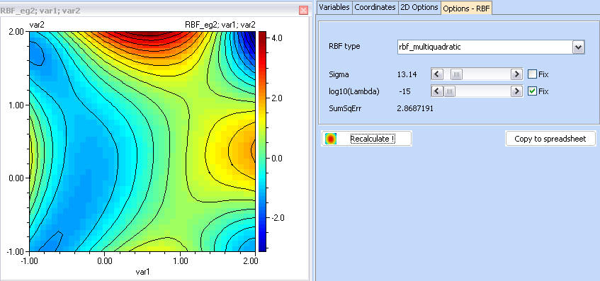
Multiquadratic f(r) = (r^2+sigma^2)^0.5 (type = rbf_multiquadratic)
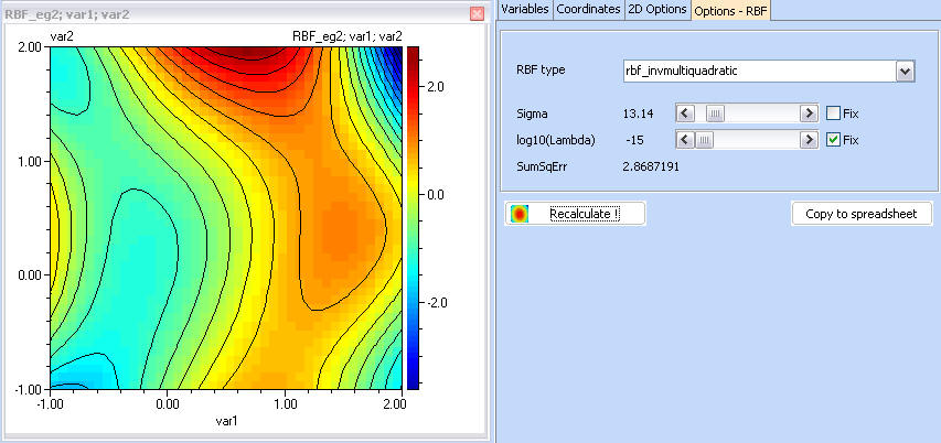
Inverse multiquadratic f(r) = (r^2+sigma^2)^(-0.5) (type = rbf_invmultiquadratic)

Additional model fields:

rbf_sigma - the sigma parameter (see above) - varies between 0.01 and 100. If sigma is undefined - then it is being internally tuned for RBFs that require it.
rbf_lambda - regularization factor - varies between -15 and 2 and is used to improve ill-conditioning by adding 10^lambda to the diagonal of the distance matrix. This parameter can be added to the model definition or tuned using the Contours and Surfaces module. The settings are on the Options_RBF tab. By removing the 'Fix' checkbox, this parameter will be automatically tuned every time the user operates with the RBF type combobox.

Usage will be shown with the eg2 model located in OptimizationModels.qsl

1. Follow the instruction in the User data evaluation example to create an input/output dataset so that you have the following:

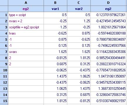
2. Use the model editor or directly type into a column the following model definition:

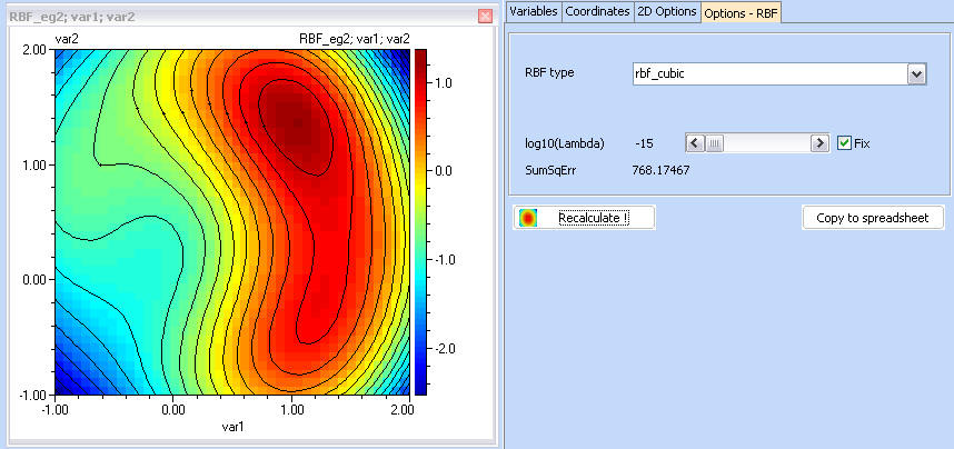
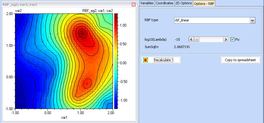
3. This RBF model is now ready to use. Let's plot contour plots and try various RBF types. (click Recalculate! to refresh the plot, after selecting a new RBF type)

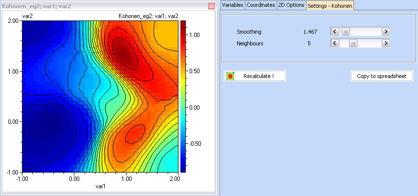
For comparison, the following is the plot obtained using the Kohonen networks:

... and using Regression polynomial (4th order, stepwise regression, R-sq=0.929, R-sq(adj)=0.909); and also Kriging;

This is the real eg2 function.

Models used for comparison

It is obvious that all models need further refinement, but at this stage, kriging produces the best results, with RBF_cubic coming after it. Looking at the theory of RBFs and Kriging, one will find that these methods have a lot in common. However because Kriging requires more computational efforts, which with the increase of the dimensionality and the number of points could become significant, RBFs are considered as a cheaper alternative, as they work in similar manner, but do no require expensive tuning.