Tutorial on model definition, optimization and robust design

(file OptimizationModels.qsl)

TASKS:

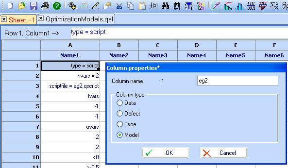
1. Open file OptimizationModels.qsl, which is located in the ‘examples’ directory within your QstatLab folder (for example C:\QstatLab\ENG5\examples\OptimizationModels.qsl). Choose one of the models copy and paste it to a new file. Name that column and specify its type as ‘model’.

2. Plot contour and 3D plots.

3. Find the minimum (maximum). Try different optimization methods and sequences. Which is the best optimization strategy? Outline the one that finds the extremum in least number of iterations. Record the optimal function and variable values.

4. Build a design of experiments. Use these experiments to build kriging and regression models. Can you say which one is the most suitable for the chosen function?

5. Compare contour plots of the kriging or regression models with the real function contours. Perform additional experiments to make these models more accurate. How would you choose where to place the new experiments? Use kriging_mse if you have built a kriging model or D-optimal design of experiments if you have used regression model. What is the minimum number of experiments required to model this function?

6. Build a stochastic model for the mean and variance. Use the analytical approach for 2^nd order regression models. For all other types, use Taylor2.

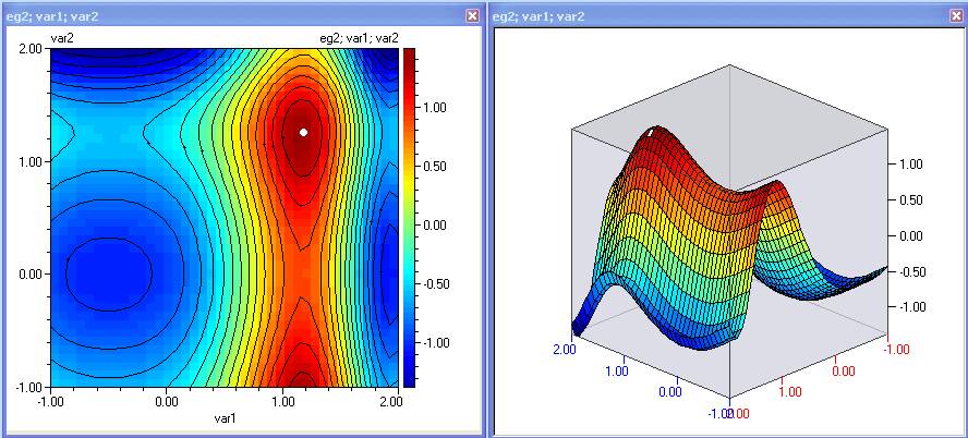
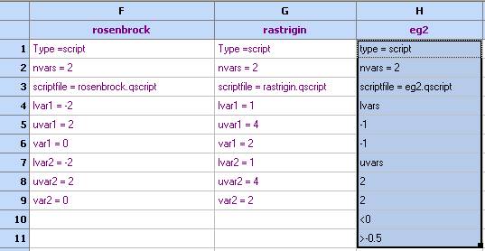
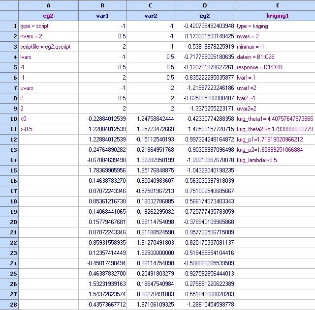
eg2

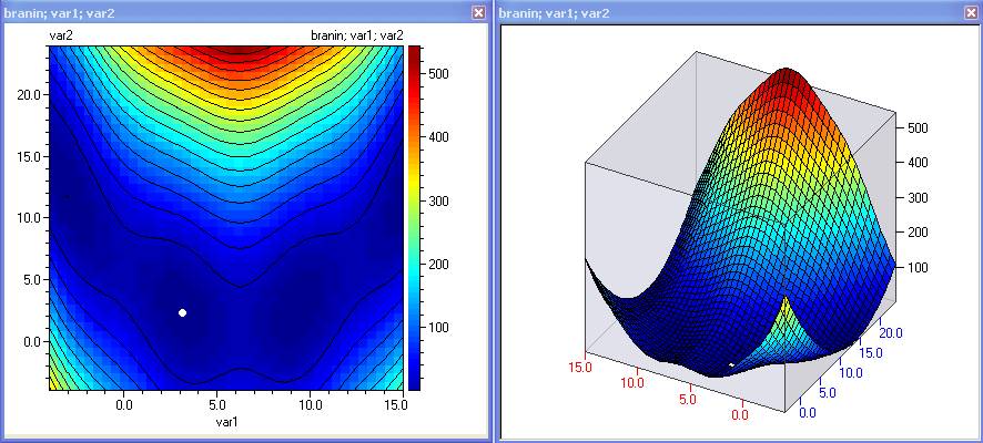
branin

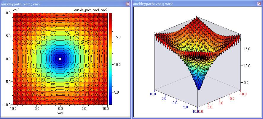
auckleypath

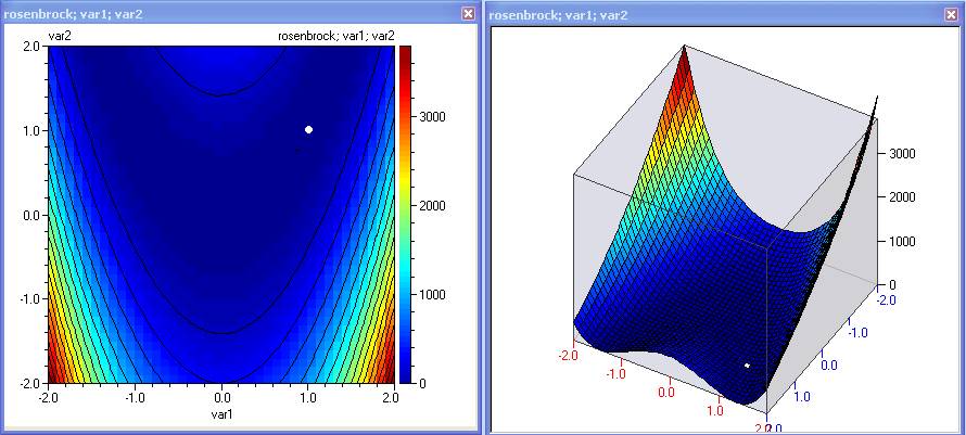
rosenbrock

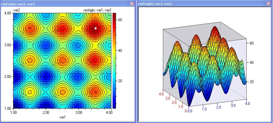
rastrigin

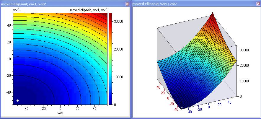
moved ellipsoid

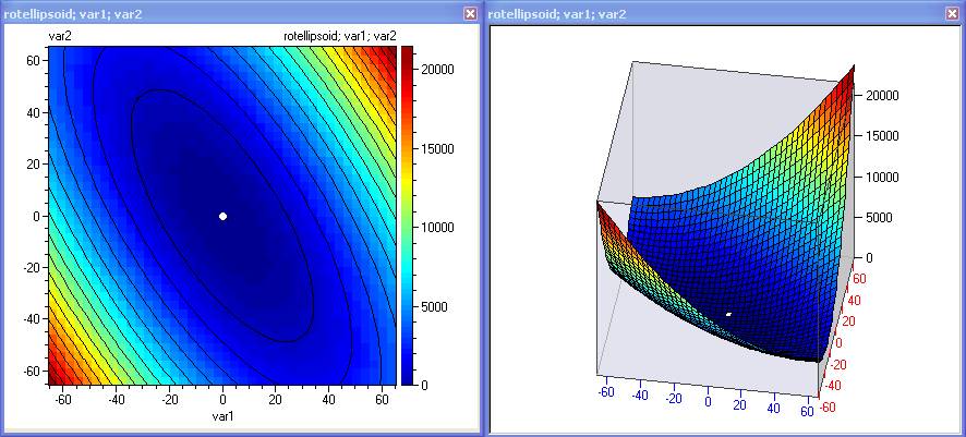
rotated ellipsoid

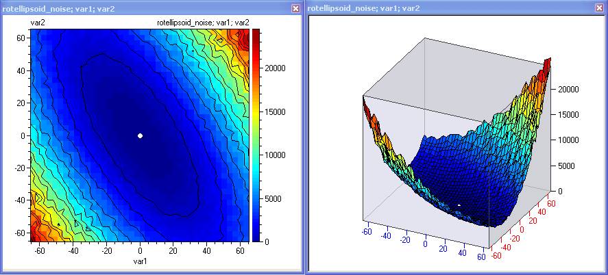
rotated ellipsoid with noise

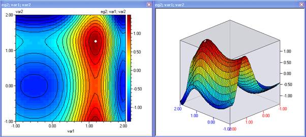
Example: Function eg2

Contour and 3D plots

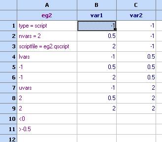
1. Open file OptimizationModels.qsl and copy function eg2 into a new Spreadsheet:

2. Use Column properties to specify name and type:

3. Close the spreadsheet called OptimizationModels and save the new file as t1.qsl

4. Plot contour or 3D plots – from the Charts/Contour plots menu.

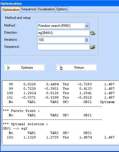
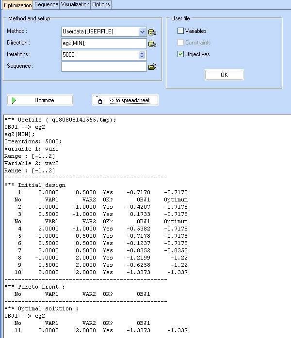
5. When the plot appears, use the ‘Optimization’ button

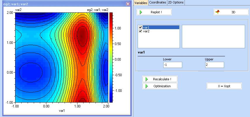
6. Specify the direction of search to be MAXimum

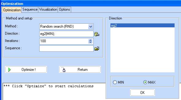
7. Click ‘Optimize!’ and after it is completed, choose ‘Visualization’ tab to see graphical representation of the results.

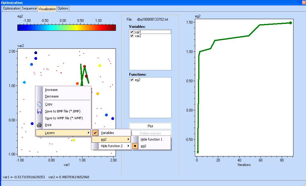
8. Use the ‘Return’ button in ‘Optimization’ section to transfer the results back to the contour plots.

9. Check the ‘Show these results on the plot’ option and specify a white colour of the optimum. Click ‘Replot !’.

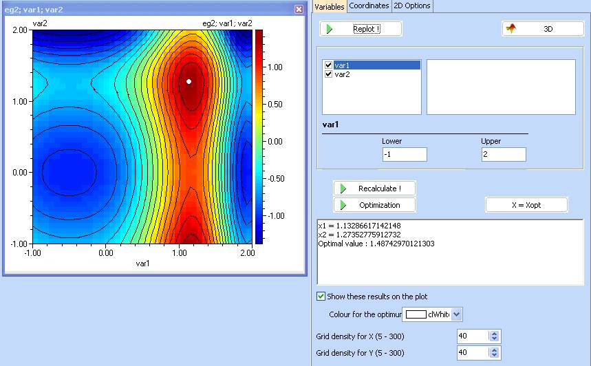
10. Repeat from step 4, using different optimization methods and initial values of the variables. Compare the accuracy and the number of required function evaluations. Note that the performance results are problem specific and will differ if applied to another function. Consult with us if in doubt.

Kriging model

(continuing with function eg2 as an example)

1. Construct a Design of Experiments. Charts / Design of Experiments. We shall use a full factorial design with 3 levels for each variable.

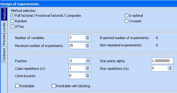
2. Change to the ‘Levels’ tab and right click in the first table. Select eg2. This will copy the number of variables and their limits from the model definition.

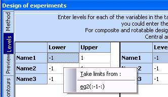
3. Enter ‘3’ in the ‘N of levels’ column for the two variables. Note that the values of the levels adjust automatically. It is possible to enter them manually, directly in the table.

4. Go to the ‘Preview’ tab and click ‘Generate’ or ‘Start’

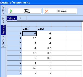
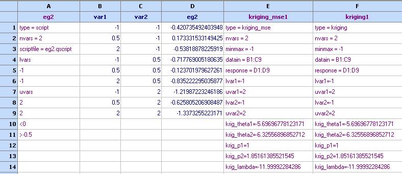
5. Click the ‘-> to spreadsheet’ button to transfer the above design to the spreadsheet then close the DOE module:

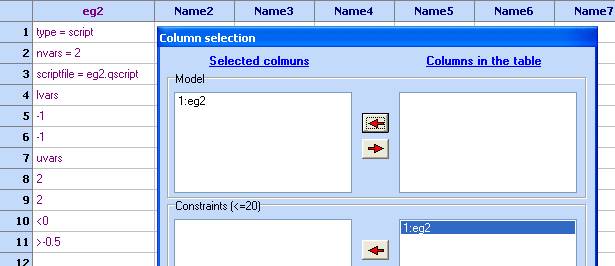
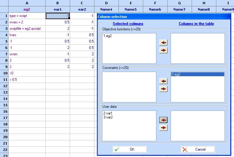
6. Compute the function values at the design points. Use the ‘Optimization’ module and choose the columns as follows:

Click ‘OK’ and then ‘Optimize!’. Use the ‘-> to spreadsheet’ button to transfer the result into the spreadsheet and choose OK.

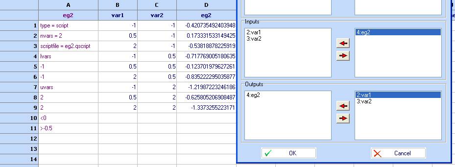
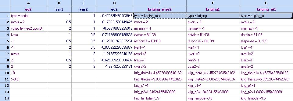
Build a kriging model (‘Charts/Kriging’), using ‘var1’ and ‘var2’ as Inputs and ‘eg2’ as an output: Click OK.

Click ‘Calculate’ and wait for the tuning to finish (the progress bar should disappear). There are 4 tuning cycles set by default.
Once the tuning is complete, use the ‘Copy to spreadsheet’ button to transfer the models back to the spreadsheet. Use the right mouse button to select which model to transfer. Once you have made your choice, use the left mouse button directly on the ‘Copy to spreadsheet’ button to actually transfer the model.

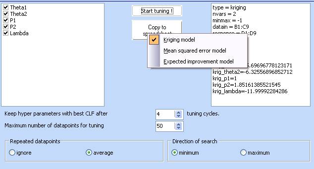
Copy the kriging model as well as the Mean squared error model.

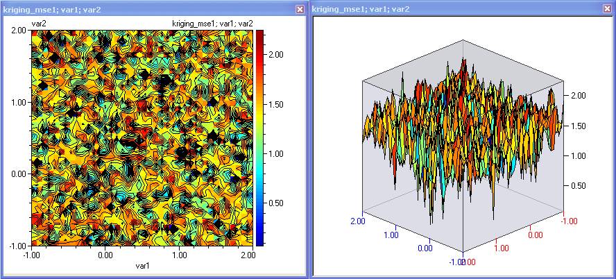
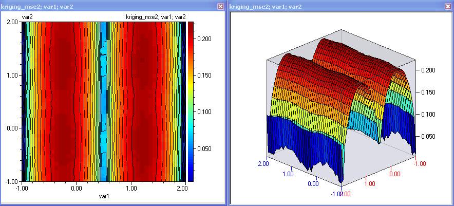
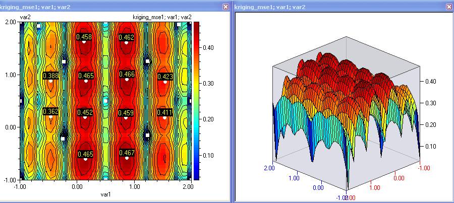
Plot contour and 3D diagrams for the Mean squared error model. Remember – theoretically this error should be 0 at the design points and increase in between. The further we are away from any design points, the higher would be the value of the prediction error. If they appear as follows, this would indicate a numerical instability during the tuning process due to matrices being close to singular. Please note that whilst the full factorial design is best for building regression polynomials, it might not be the best choice for kriging models.

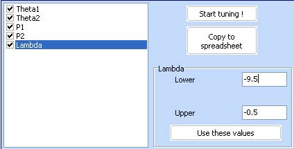
13. To avoid numerical instabilities when they occur, we could increase slightly the lower bound of the Lambda parameter, which would have a regularization effect. For this demonstration – we have chosen a lower bound of -9.5. Make the change in the Kriging module, click ‘Use these values’ and then repeat the tuning.

14. Once the new tuning is complete, transfer the MSE model and make sure that it now looks as follows:

Now transfer the other two models (see step 9). Note that they differ only by their first rows.

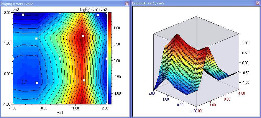
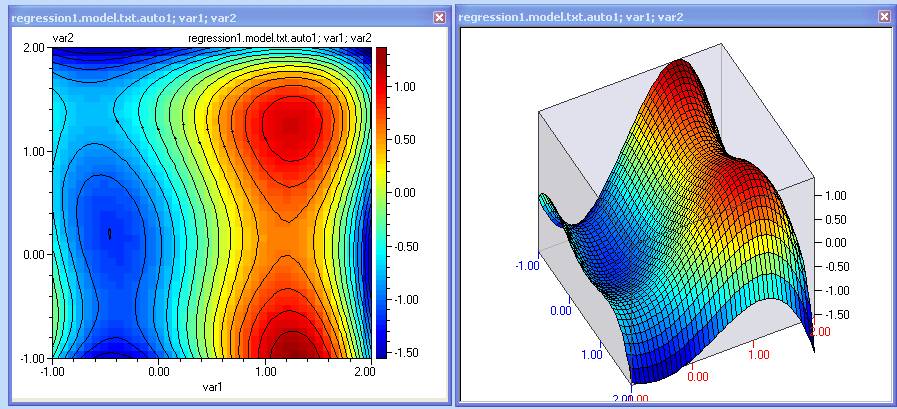
Plot contours for ‘kriging1’. This is the model that predicts the value of eg2 at the design points.

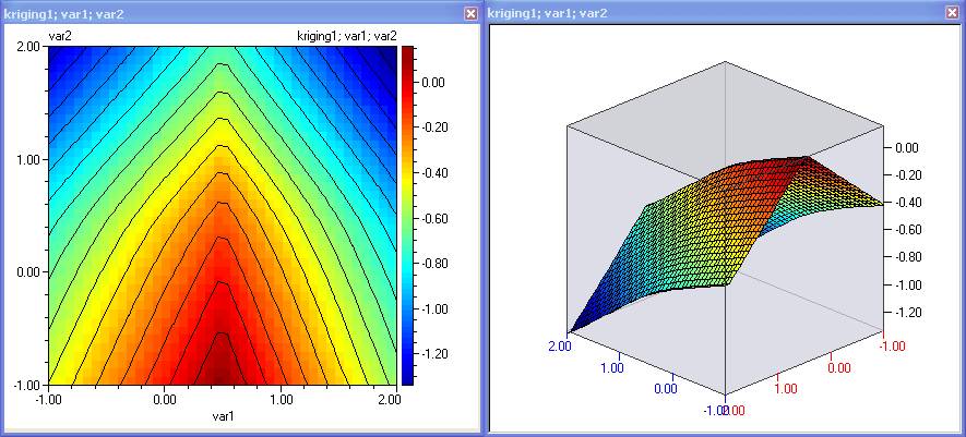
Comparing these plots with the original function shows that although the kriging predicts accurately at the design points, the space between them is highly interpolated. When modelling previously unknown functions, it might not be possible to visually compare observed and predicted plots. In this case – cross validation is applied, where the model is calculated at several points which did not participate in the building of this model. The results from prediction and observation are the compared. If they differ, the new experiments are carried out, models re-tuned and compared again. This continues until the models predict accurately after cross-validation.
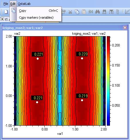
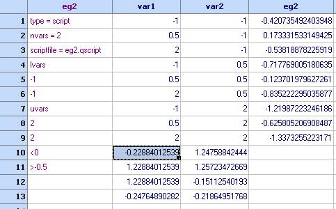
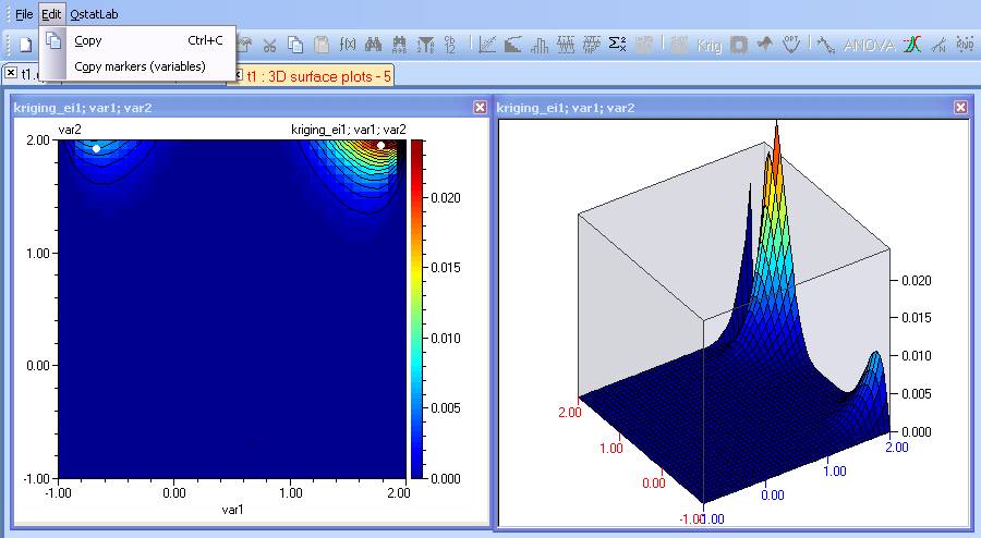
As we have identified, the current prediction is not sufficiently accurate. Therefore we now need to select locations for new experiments. Logically one would like to add more information where it is missed the most, which is indicated by the maximum values of the MSE. Plot contours for kriging_mse2 and whilst holding the CTRL key down, click to mark the locations of the maximum error. Then use Edit/Copy markers (variables):

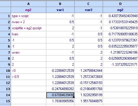
Go back to the spreadsheet, select a cell below the design points and paste the copied values there:

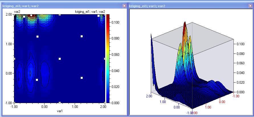
In some cases it is useful to add experiments which maximize the expected improvement function. By default it will be maximum where it is most likely to find a minimum. If we are searching for maximum then this can be specified in the kriging module, and then the expected improvement will be maximum where it is most likely to find a maximum of the function. Therefore we repeat the point selection, using kriging_ei1’.

Then add these points to the design of experiments.

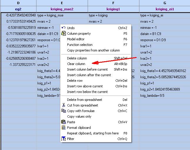
Clear (but do not delete) the columns that contain the function values and the kriging models to prepare them for a second iteration.

Repeat from step 6.
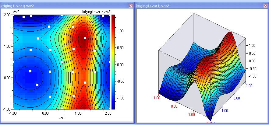
Continue until reaching a satisfactory level of accuracy, depending on the purpose of the model. After the second iteration we have achieved this:

23. It is seen that for the purpose of optimization, this model is good, as there are sufficient experiments around the extremums indicating that the prediction in these areas is accurate. Should we wish to further update the model, we can select new set of points which maximize the MSE (and/or IE).

Do the same with the IE function, which now has a well developed maximum at the location of the minimum of the objective function. Mark them, transfer to the spreadsheet:

Evaluate the function at the new points and build new kriging model (step 21). Contours of the prediction after the third iteration look as follows:

These contours now look very much like the originals, which indicates that the model is good for prediction / optimization purposes. A 4^th order regression polynomial built on the same data looks as follows:

Continuing with D-optimal design and building new regression models would make an interesting research exercise.

Robust design

(continuing with function eg2 as an example)

Now that we have an accurate kriging model we can use it for optimal robust design. This is not feasible without a RSM (response surface model) due to the time, number and cost of function evaluations.

Clear all columns, except those that contain the data and the kriging model

Important !!! Please have in mind that the data used to tune a kriging model is always part of the model itself. They are referenced in the following fields: datain and reponse. Model prediction will not function properly if the data cannot be found in the location specified in these two fields.
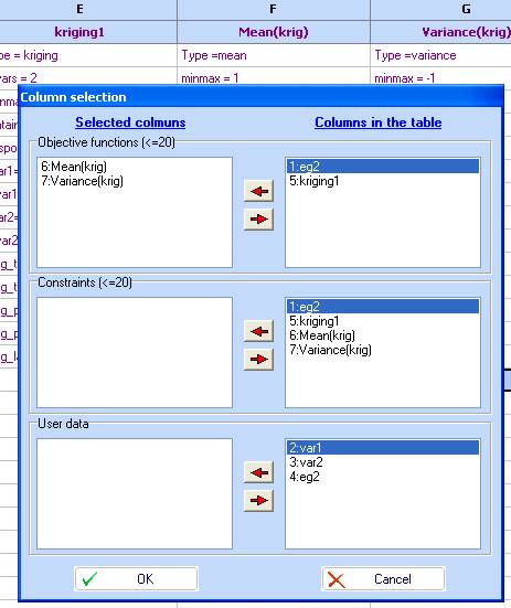
Let’s create stochastic model representing mean and variance. Click in column F and then activate the ‘Model editor’ (in the Edit menu). Fill the fields as follows:

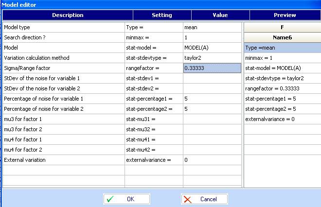
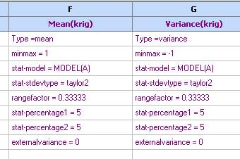
Click OK and the model will appear in the spreadsheet. Click in column G and repeat the above but setting the model type to ‘variance’ and the search direction to (-1: minimum). Transfer this model to the spreadsheet and change their names (Column properties):

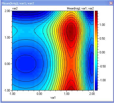
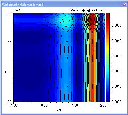
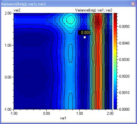
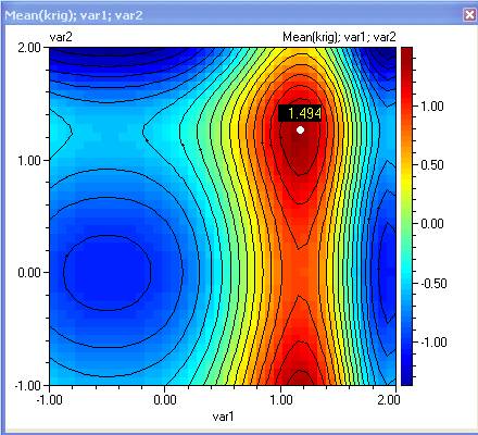
Plot contours for the mean and variance. Can you visually spot the optimal robust solution? It would be the one that maximizes the mean and minimizes the variance.

When visual plots are not feasible, use Multiobjective optimization Start the ‘Optimization module’ with the following selection:

Change the search direction for the Mean to MAX, click ‘OK’ and then ‘Optimize!’

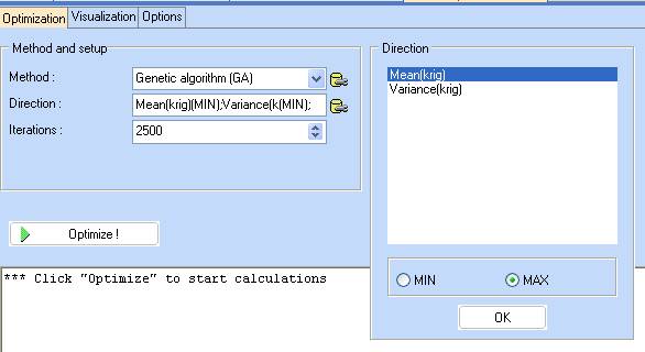
Once optimization is completed, change to ‘Visualization’. We observe that there are 4 points with minimal Variance. Holding the CTRL key down, set markers at each one of them. The one of most interest would be number 1, as it has maximum Mean.

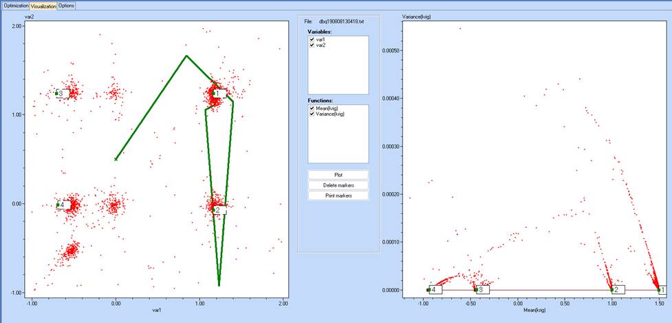
Detailed information on the marked points can be found at the bottom of the text screen (Within section ‘Optimization’)

*** Optimal solution :

OBJ1 --> Mean(krig)

OBJ2 --> Variance(krig)

No VAR1 VAR2 OK? OBJ1 OBJ2

2552 1.1782 1.2520 Yes 1.4997 0.0000 1.5

No VAR1 VAR2 OK? OBJ1 OBJ2

886 1.1669 1.2409 1 1.4986 0.0000 <-- Marker 1

579 1.1673 -0.0727 1 1.0017 0.0000 <-- Marker 2

2368 -0.7063 1.2377 1 -0.4352 0.0000 <-- Marker 3

546 -0.6942 -0.0146 1 -0.9363 0.0000 <-- Marker 4

By manually placing a marker at the optimal location on the contour plot we can see that in this case, the maximum is a robust solution, because the Variance is 0. :