Contours and 3D plots
Required data
You need at
least one column containing a model definition. See models.
We will be using model stored in file models.qsl, supplied in the examples
directory.
- For this example, we have used the Spreadsheet model.
- On the 'Variables' tab, you can choose to
display 3D or 2D plots.
- You can choose which two variables to show
the contours for. Variables chosen for plotting can have custom upper and
lower bounds. Others will be kept constant. The constant value can be
defined.
- Once the plot is visualized, the user can
choose to find the optimum value. This is especially useful if the function
has more than 2 variables and it is not obvious from the plot where the
optimum is. After optimization is complete, the results are returned. Click
"X=Xopt" to replot the graphs with the optimal values. You can choose to
show the optimal value on the plot.
- The size of the grid can be modified. The
higher the number, the smoother the plot, however this may significantly
increase computation time.
- The tab 'Coordinates' shows values of the
variables and function as the user moves the mouse over the plots
- 2D Options and 3D Options are available,
depending on which of the plots is active. To activate a plot, just click it
once.
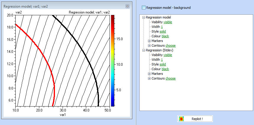
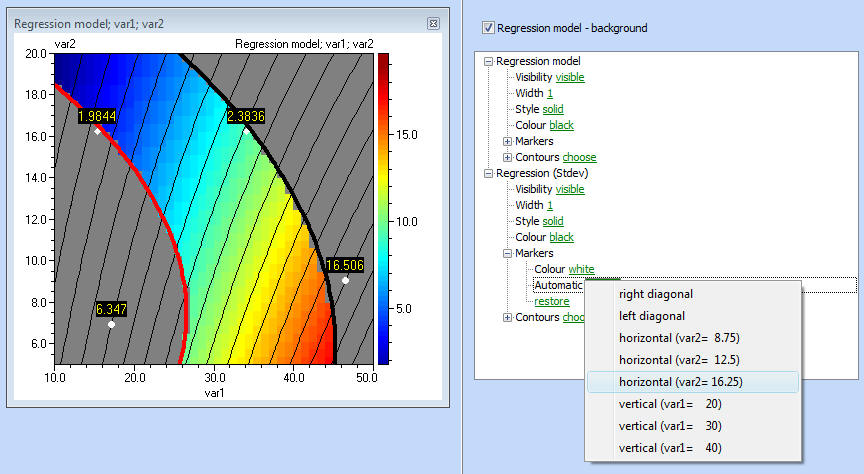
- For the 2D plots, the user may change the
appearance of the plots, by changing the number of contours, their colours,
thickness, adding markers to show contours values etc.
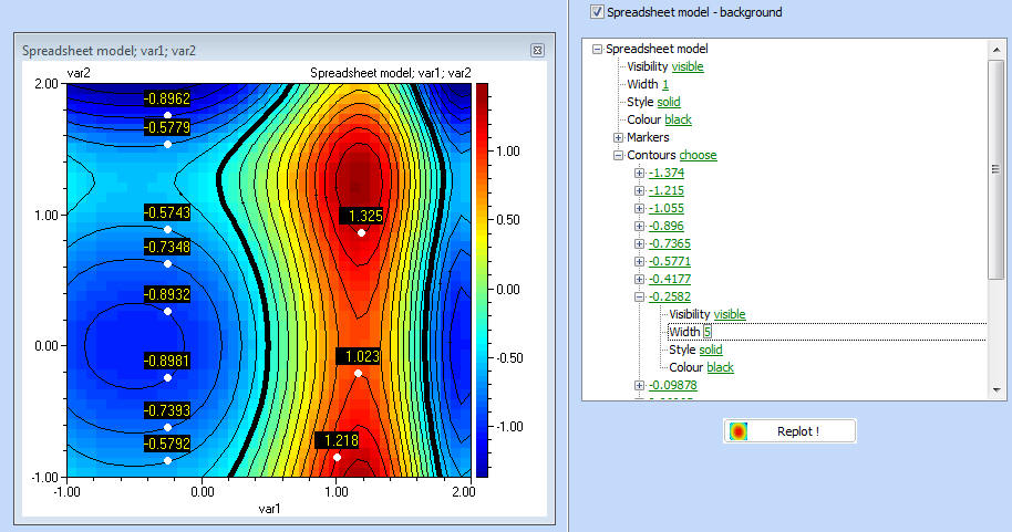
- To place a marker in a custom location, hold
CTRL and click the mouse at the location where you would like to place the
marker
- Various options are available for the 3D
plots as well. Use them to customize the view.
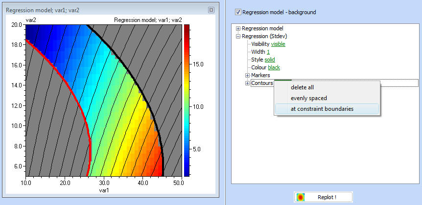
It is possible to plot more than one models at a
time. To do that, use one model for the main model and all others as
constraints.
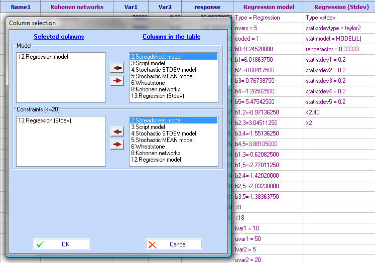
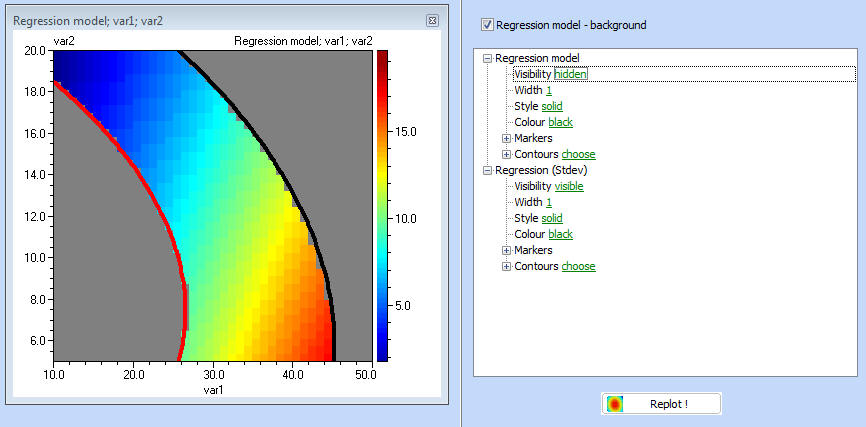
The main model will be used to plot the background. It will be gray where the
constraints are violated.
See also:
Working with discrete variables
Back to Data Entry