Working with discrete variables

In cases where one or more variables should take only predefined set of values, it is possible to define discrete variables. If a variable is defined as discrete, consequent optimization or plotting routines will use its discrete values.

We shall demonstrate this on one of the models, included in file 'examples\Optimization models.qsl'.

After locating and loading the file, clean up the file so that only the model we will be working on remains. To do that - select all models but the first, and use 'Clear column' after a right mouse click:

Only the first model remains:

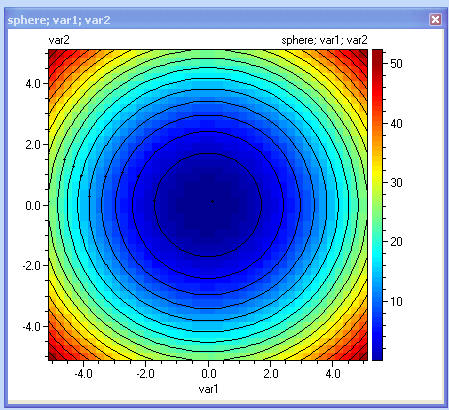
This model does not have any discrete variables defined, and therefore it will treated as continuous. As such, one can see that the minimal value is in the centre where all variables are equal to 0, and its maximums are in the corners, where the squared values of the variables are at maximum.

Now, let us assume that variable 1 can only take the following values: -5.1; 4.3; 0.4; 2.9; 4.3. We can define this by including dvar1 = -5.1; 4.3; 0.4; 2.9; 4.3 in the model definition column:

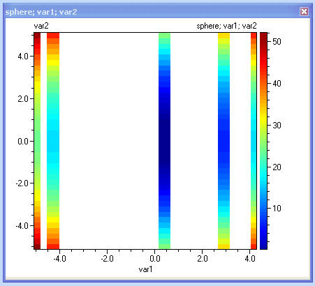
Building a contour plot of this model will only calculate the objective function at the allowed discrete values for var1 and will treat var2 as continuous.

Another way to define discrete variable is by referring it to a range of cells that contains the discrete values. This way would be more convenient if the amount of discrete values is larger. The following screenshot var2 being defined in this fashion. 

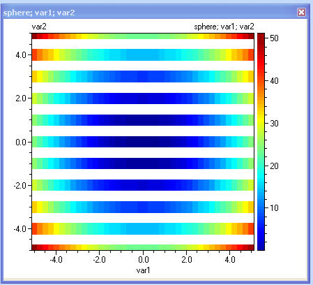
Note that in this example only var2 is defined as discrete, and therefore var1 is treated as continuous, which is shown on the following contour plot:

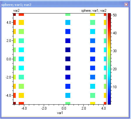
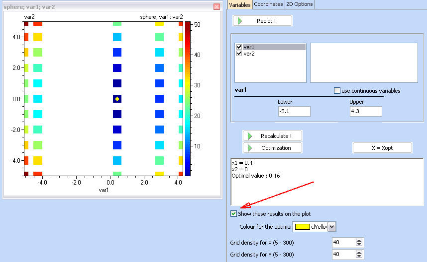
The following is a combination of the above examples. Both var1 and var2 are defined as discrete

The objective function is being calculated only in the specified discrete values.

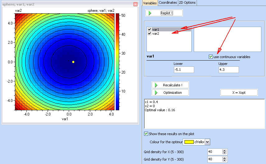
To carry on with Optimization,  use the 'Optimization button'. The following example demonstrates the use of 'Exhaustive search (SCAN)' optimizer, which scans trough the discrete values of the variables and chooses the minimum value of the objective function. Note that despite the fact that in continuous space, the optimum is 0, at var1 = var2 = 0, in this particular discrete example, the minimum is 0.16 at var1 = 0.4, var2 = 0, which obviously is due to the fact that var1 = 0 is not allowed discrete value here.

Note that the discrete variables are now denoted with (D), and only discrete values are allowed.

The visualization section, shows the optimization procedure using the discrete values.

Returning to the contour plots screen, optimization results could be shown on the plot by selecting 'Show these results on the plot'

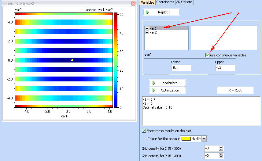
Note that contour plots allow plotting in continuous space for any discrete variable, by using the 'use continuous variables' after selecting one of the variables. The following shows this with var1

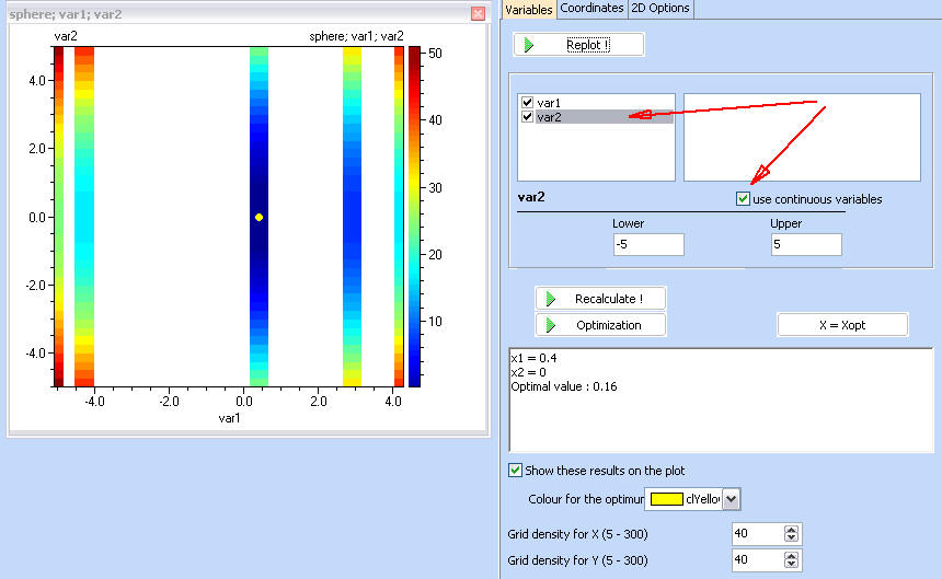
... and with var2

... and with both variables