Kriging
Implementation in QstatLab
QstatLab allows training and searching of kriging models. The training is effectively an optimization problem where the optimization parameters are the hyper parameters Theta, P and Lambda (see the theory below). For n variables, we would have 2*n+1 parameters to optimize. One can see that as n increases the number of optimization parameters can become too great to be handled by any optimization problem. In large dimensional problems, it is recommended to keep the P parameters constant with a value of 2.
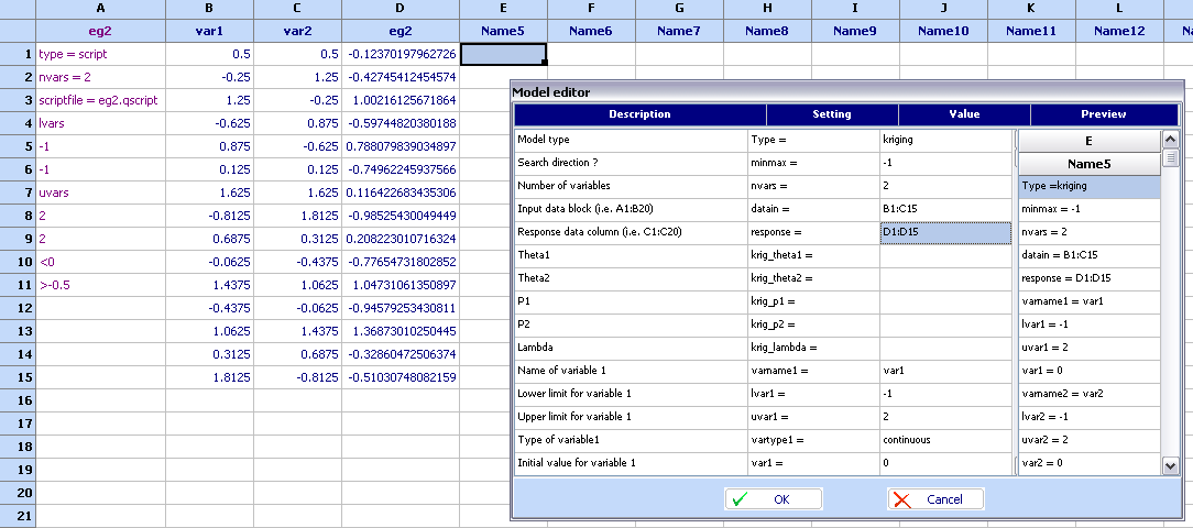
The kriging usage will be shown with the eg2 model located in OptimizationModels.qsl
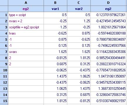
1. Follow the instruction in the User data evaluation example to create an input/output dataset so that you have the following:
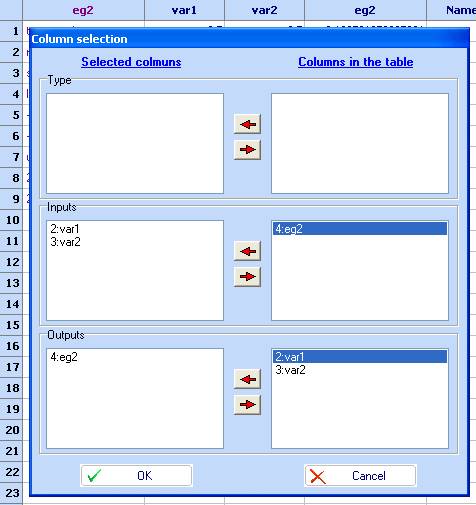
1. Select 'Kriging' from the Charts menu and specify the columns to use, then click OK
2. The kriging module will load with the following dialog
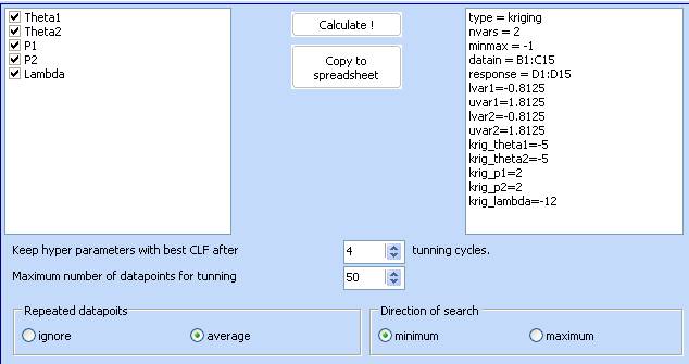
· Hyper parameters Theta, P and Lambda will be varied to maximize the CLF (concentrated likelihood function).
· Keep hyper parameters with best CLF after 4 tuning cycles. The optimization cycle can be repeated several times (4 in this case). If the optimization algorithm finds different optimal values, the module will keep the ones that give the best CLF.
· Maximum number of datapoints for tuning: When the dataset contains large number of datapoints, the tuning process might be slow. Therefore the user can restrict the maximum number of points that the system uses for tuning. The original number of data will be used during prediction.
· Repeated datapoints. When there are repeated points, the user can choose to ignore the repetitions or to average them.
· Direction of search. This is important for the calculation of the expected improvement function as it defines where does the function ‘improve’. Ignore this setting if you do not plan to use the expected improvement function.
Click ‘Calculate’ to start the tuning process.
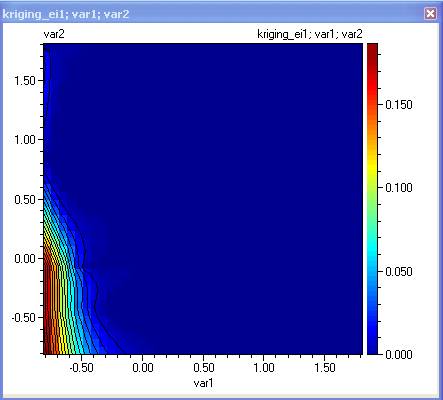
3. When the progress indicator disappears, the tuning process is completed. A short analysis of the model will be given:
Variables:2
var1
var2
Output values:eg2
Tuning using 15 datapoints out of 15
------ Tuning cycle1 -------
Hyper1 = 0.131905546305271
Hyper2 = -1.42017527958295
Hyper3 = 1.99972201956888
Hyper4 = 1
Hyper5 = -12
CLF = 15.6612629610882
------ Tuning cycle2 -------
Hyper1 = 0.147211010765128
Hyper2 = -1.46145538651498
Hyper3 = 1.99999351525317
Hyper4 = 1
Hyper5 = -12
CLF = 15.6458475168103
------ Tuning cycle3 -------
Hyper1 = 0.117525302837744
Hyper2 = -1.44307362994341
Hyper3 = 1.99997813880588
Hyper4 = 1
Hyper5 = -12
CLF = 15.6616163848123
------ Tuning cycle4 -------
Hyper1 = 0.154750423397989
Hyper2 = -1.32675896340584
Hyper3 = 1.99999985254462
Hyper4 = 1
Hyper5 = -12
CLF = 15.6365699449969
observed predicted residual error exp.improvement
------------------------------------------------------------------------------------
-0.12370198 -0.12370197 -9.5405759E-9 3.265011E-7 1.2554041E-7
-0.42745412 -0.42745411 -1.303539E-8 4.4605398E-7 1.7150808E-7
1.0021613 1.0021611 1.2336649E-7 4.2216574E-6 1.7465999E-6
-0.5974482 -0.59744818 -2.0019345E-8 6.8477189E-7 2.6329152E-7
0.78807984 0.78807981 3.1233358E-8 1.0683336E-6 4.4200226E-7
-0.74962246 -0.74962245 -1.3482544E-8 4.6136943E-7 1.7739709E-7
0.11642268 0.11642268 4.8873919E-9 1.6716323E-7 6.9160677E-8
-0.9852543 -0.98525427 -3.3893017E-8 1.1596056E-6 4.4586676E-7
0.20822301 0.208223 6.0201221E-9 2.0600683E-7 8.5229984E-8
-0.77654732 -0.77654729 -3.0157146E-8 1.0314757E-6 3.9659655E-7
1.0473106 1.0473106 5.5662852E-8 1.9045944E-6 7.8797911E-7
-0.94579253 -0.94579254 8.4189272E-9 2.8811823E-7 1.1920107E-7
1.3687301 1.36873 6.5024793E-8 2.2246464E-6 9.20397E-7
-0.32860473 -0.3286047 -2.2139825E-8 7.5771561E-7 2.9134391E-7
-0.51030748 -0.51030742 -6.2123293E-8 2.1258001E-6 8.1737199E-7
Total residual 1.7579408004062E-7
Observed – the value from the dataset
Predicted – the value calculated using the trained kriging model
Residual – the difference between Observed and Predicted
Error – the root of the Mean Squared Error calculated at this point by removing this data from the data set used for prediction
Exp.improvement – the probability of improvement (in terms of optimum)
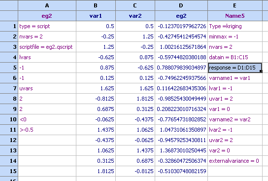
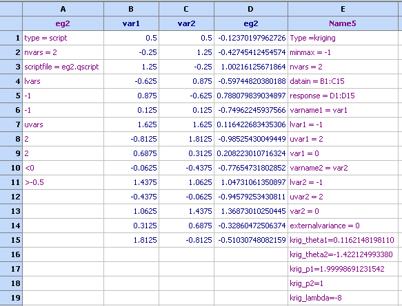
4. Three models are now available.
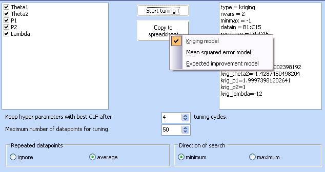
Select each one of them and then click the ‘Copy to spreadsheet’ button. The models will be transferred to the spreadsheet.
Please note that when these models are being used, they will need to refer to the data specified in ‘datain’ and ‘reposnse’ fields. Therefore these data needs to be available at calculation time.
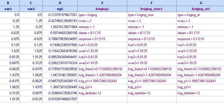
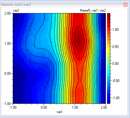
These models are now ready for further use in optimization or contour plots studies. Their contours are as follow
The prediction:
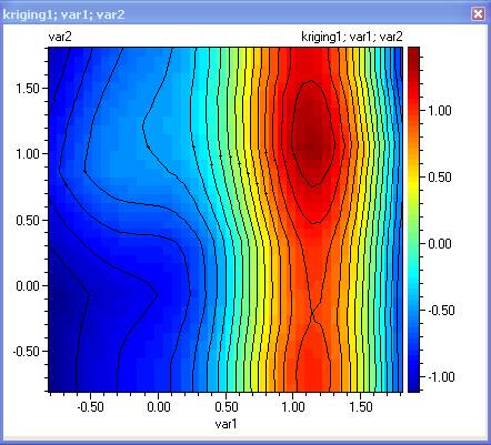
The prediction error – this plot can be used to plan further experiments where the error is greatest. Use CTRL + mouse click to set markers at the locations of maximum error and then use the Edit/Copy markers (variables) to copy the coordinates of the marked points. They can then be pasted to the spreadsheet.
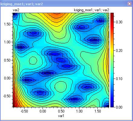
Expected improvement. This function has its maximum where it is most likely to find the minimum of the function. The user would plan at least one new experiment at the maximum of this function if the function is being used for optimization purposes.
Kriging model can also be defined directly from the Model editor:
The most vital fields are nvars, datain and response. Note that the theta, p and lambda have been left empty. And the model looks as follows:
Any attempt to use this model, will lead to automatic training of the hyper parameters. If any of the hyper parameters are specified then they will keep their value as constant but the ones that are not defined will be trained. This can be demonstrated for instance by plotting a contour plots of the 'Name5' model:

Choosing 'Yes' will store the hyper parameters, so that next time they will not be trained again.
The resulting plot is similar to the one obtained above:
See also:
Tutorial on models, optimization and robust design
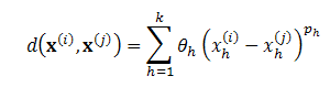
The relationship between inputs x and observations (responses) y is expressed as
![]()
where ![]() represents the
function or process which will be interpolated.
represents the
function or process which will be interpolated.
We evaluate this response for combinations of inputs representing our experimental design and use this information to construct an approximation
![]()
The response at x is expressed as
![]()
where ![]() is the mean of the
input responses and
is the mean of the
input responses and ![]() is a Gaussian random
function with zero mean and variance
is a Gaussian random
function with zero mean and variance ![]() . We do not assume
that the ε are constant as in regression, but that these
errors are correlated. The correlation between two points being related to some
distance measure between corresponding points. The distance measure used here
is
. We do not assume
that the ε are constant as in regression, but that these
errors are correlated. The correlation between two points being related to some
distance measure between corresponding points. The distance measure used here
is
where ![]() and
and ![]() are hyperparameters
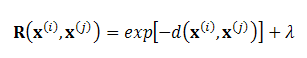
yet to be determined. The correlation between points x(i) and x(j)
is defined by
are hyperparameters
yet to be determined. The correlation between points x(i) and x(j)
is defined by
![]()
An additional hyper parameter could be a regularization term added to the diagonal of R, denoted as l:
When we wish to sample at a new point x, we form a vector of correlations between the new point and the previously sampled points
![]()
If x is close to x(i), then these points are correlated and the predicted response will be strongly influenced by the response at x(i). Whereas if the points are far apart, the correlation is small and the predicted response will only be weakly influenced by the response at x(i).The prediction itself is given by
![]()
where the mean μ is defined by
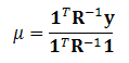
Hyper
parameters ![]() and
and ![]() and l are obtain by maximizing the concentrated likelihood
function given as follows:
and l are obtain by maximizing the concentrated likelihood
function given as follows:
CLF =
where the
variance ![]() is given by
is given by
Another useful quantity is the mean squared error (MSE) of prediction
as this gives us a measure of the accuracy of our prediction at x. If the kriging model is used for optimization purposes, another useful quantity called Expected improvement can be computed:
See also:
Tutorial on models, optimization and robust design