General procedure - single objective optimization
Use Charts/Optimization to select models for optimization. Alternatively, the tool can be started from the Contour plots. The optimization procedure will be described using the Goldstein - Price as an example, which is located in models.qsl. (If you get a message that the value across the variation range is constant, go back to the spreadsheet and click 'Recalculate'). The function looks like this:
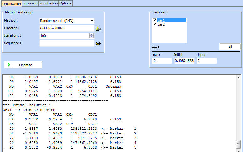
After invoking the Optimization tool, you first need to choose optimization method, number of iterations and direction. Some methods such as Genetic algorithms and Gradient methods have additional settings, which are preloaded with the most used values.
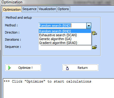
The variables section on the right, provides additional control. It is possible to choose which variables should be changed during the process and which should be the range for changing them. When setting upper and lower limits, it is possible to propagate these values to all of the variables, by clicking 'All'.
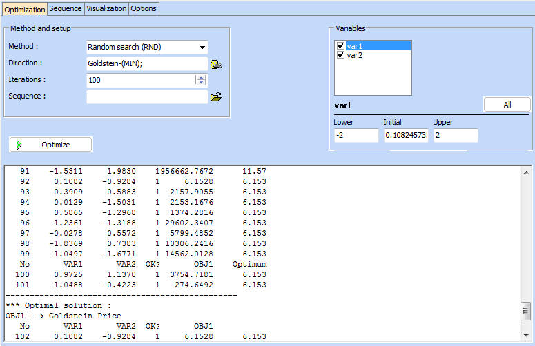
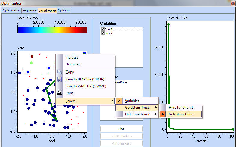
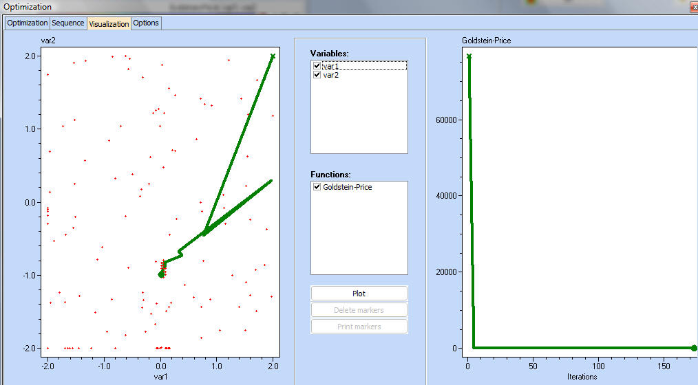
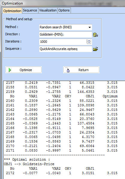
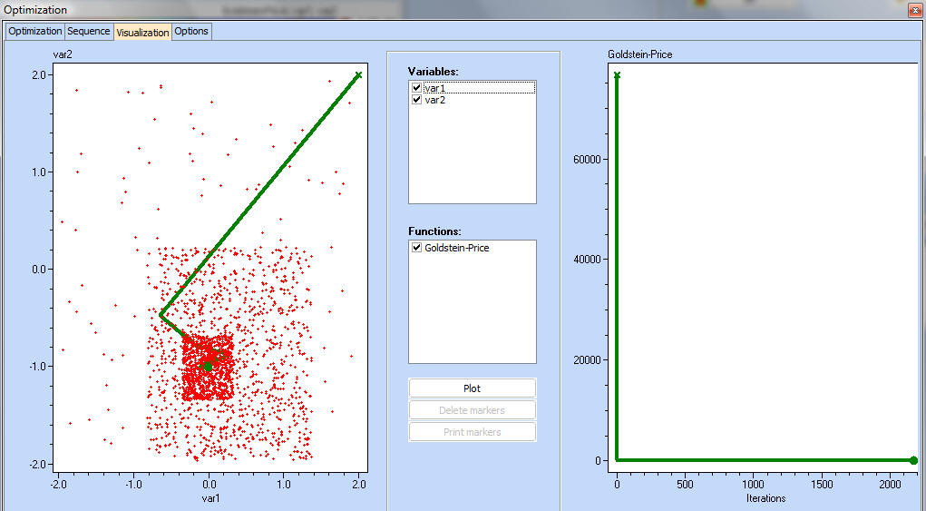
Click the 'Optimize' button to start the optimization. Information for each iteration will be displayed. The first column is iteration number, followed by variables, constraints, feasibility and objective functions. The last column is the best value for the first objective found so far. Once the optimization process is complete, it is possible to examine the optimization progress in the 'Visualisation' Tab. A cross denotes the start of the process and a circle - the final point.
By removing the thick on the 'Optimal trace only - function' we can show all values of the objective function:
By holding the CTRL key and clicking on any of the two plots, the user can set visual markers. If a marker is set on the left plot, it will appear on the right one as well and vice versa.
Marker values appear on the 'Optimization' tab at the bottom of the log screen
Both plots can be zoomed in or out, using the popup menus (Increase and Decrease) options. On the variables plot it is possible to show only the location of the design point, but also some information about the value of the function at arbitrarily selected points, using colour coding.
After each optimization cycle, it is possible to change the settings and methods and repeat the procedure. The last point from previous optimization will become initial point for the next.
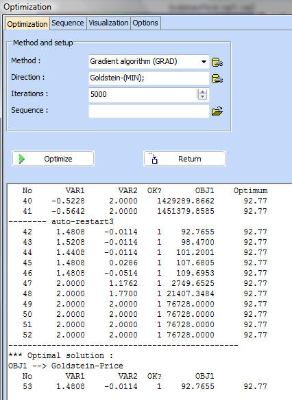
With some functions it is efficient and convenient to combine several methods in a sequence and therefore to exploit the strengths of each method. For instance, using the Gradient search on its own on the Goldstein-Price function, leads to a minimum of 92.77, (whilst the real minimum is 0). The reason for this is the fact that close to the minimum, the function has very low gradient values and therefore, the Gradient search stalls.
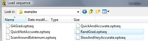
Several pre-programmed sequences are available in the examples directory. The file with a sequence should be chosen in the 'Sequence' field. Choose 'RandGrad.optseq' which in effect is a sequence of Random search, followed by a Gradient search.
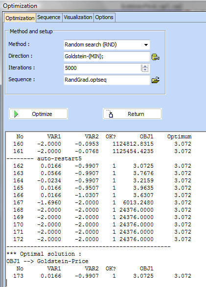
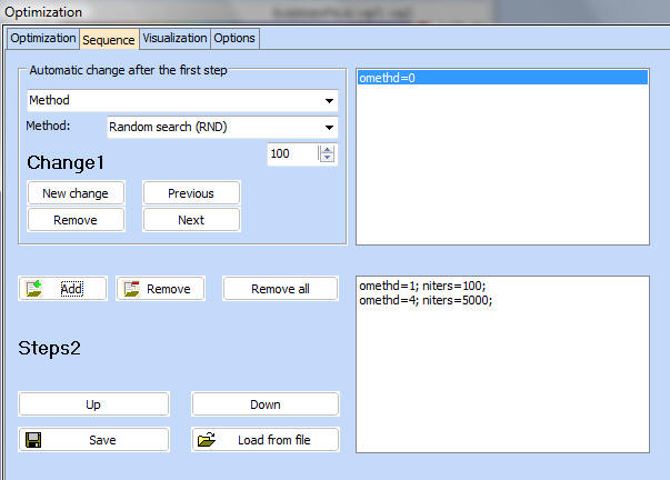
It is obvious that the combination of the two methods, produced a result much closer to the real optimum. The sequence tab allows constructing or editing sequences. Each new STEP copies the settings for the previous STEP and applies the specified changes. For instance in the RandGrad.optseq sequence, it is specified that the first STEP consist of random search (OMETHD=1) for 100 iterations and followed by Gradient method (OMETHD = 4) for maximum of 5000 iterations.
In the Visualisation, it is illustrated the path to optimum. One can see the random points and the Gradient probing around the minimum. This is often an efficient combination, as random search can quickly identify the vicinity of the optimum and the gradient search can home in on the minimum more accurately by keeping the number of function evaluations to minimum.
The 'ScanAroundExtremum' sequence represents a combination of two exhaustive searches, where the bounds for the variables narrow around the previously found minimum.
This is the contents of the sequence file, used to produce the plots above:
omethd=2; nsteps=5; autolimits=50; autolimitsstyle=1; niters=10000000;
omethd=2; nsteps=10; autolimits=50; autolimitsstyle=1;
QstatLab will first execute the method specified on the 'Optimization' tab. In this case by default we have Random search for 100 iterations. Then it will proceed with the specified sequence, listed above. The method will change to 2 (Exhaustive search), with number of steps within the factor interval. The interval will be reduced by 50% of the previous bounds. Maximum number of iterations is 10000000. Next, the number of steps is increased and the limits are further reduced by 50% of the preivous. The autolimitstyle defines if we want to increase the bounds or decrease them.
Here is an example of another sequence: Quickandaccurate.optseq.
The sequence file contains the following lines:
omethd=1; niters=1000; autolimits=55; autolimitsstyle=1;
autolimits=55; autolimitsstyle=1; nsteps=8; omethd=2; niters=1000000;
omethd=1; niters=1000; autolimits=55; autolimitsstyle=1;
Starting with the random design for 100 iterations, limits are reduced by 55% of the previous - three times, and alternating methods 1 and 2 - random and exhaustive searches. It is seen that the global optimal has been found with great precision with the expense of 2171 iterations.
See also