
Normality test
Many of the statistical methods are based on the assumption for normality of observations. In QSTATLAB this assumption is tested through the Anderson-Darling method. It uses so called normal probability plots to compare the data with the theoretical distribution. The scale of this plot is so chosen that if the data are normally distributed they are arranged on a straight line on the plot.
Example The table below shows data for the height x (centimeters) of 30 pupils. Check if the distribution of x is normal.
Height of pupils
|
№ |
x |
№ |
x |
№ |
x |
№ |
x |
№ |
x |
№ |
x |
|
1 |
157,9 |
6 |
166,4 |
11 |
155,4 |
16 |
156,2 |
21 |
158,8 |
26 |
158,9 |
|
2 |
158,8 |
7 |
157,1 |
12 |
170,4 |
17 |
142,3 |
22 |
156,0 |
27 |
160,5 |
|
3 |
169,3 |
8 |
147,9 |
13 |
168,9 |
18 |
150,2 |
23 |
154,7 |
28 |
165,0 |
|
4 |
163,6 |
9 |
156,0 |
14 |
156,0 |
19 |
158,0 |
24 |
171,9 |
29 |
175,5 |
|
5 |
140,3 |
10 |
149,9 |
15 |
146,2 |
20 |
154,9 |
25 |
164,6 |
30 |
171,8 |
Fragment of data for normality test
Click
“Charts”
menu or the icon for
normality test
 ,
select column,
then click OK and the normal probability plot
will appear. One can see that the height of
the pupils can be considered as normally distributed random variable.
,
select column,
then click OK and the normal probability plot
will appear. One can see that the height of
the pupils can be considered as normally distributed random variable.

Normal plot for height of pupils
Below the plot are shown values AD and p, as well as number of data (30), mean (158.8) and standard deviation (8.8). When AD is small and p is reasonably large (usually p >0.1) the normality assumption is accepted. In this example we can accept that the data are approximately normally distributed.
Another plot which shows the probability of observations to be normal as function of the random variable is given below.

Probability of observations as function of the random variable under normality assumption
Example. The table below shows 30 values of particle size (mm) obtained in a process of fragmentation. Let's test them for normality.
Size of particles (mm) obtained by fragmentation
|
№ |
x |
№ |
x |
№ |
x |
№ |
x |
№ |
x |
№ |
x |
|
1 |
0.5 |
6 |
4.8 |
11 |
5.9 |
16 |
6.6 |
21 |
4.9 |
26 |
9.9 |
|
2 |
3.5 |
7 |
1.8 |
12 |
1.5 |
17 |
0.9 |
22 |
11.0 |
27 |
1.4 |
|
3 |
4.9 |
8 |
5.0 |
13 |
3.8 |
18 |
0.8 |
23 |
1.2 |
28 |
1.4 |
|
4 |
5.7 |
9 |
0.7 |
14 |
1.3 |
19 |
9.2 |
24 |
1.8 |
29 |
1.6 |
|
5 |
1.6 |
10 |
1.1 |
15 |
1.4 |
20 |
2.5 |
25 |
1.9 |
30 |
1.4 |
The figure below shows that they are not normally distributed because the points do not lie on a straight line, AD is large and p is very small (p<< 0.1).

Normal plot for size of particles obtained by fragmentation
Another view shows the probability of observations as function of the particle’s size under normality assumption.
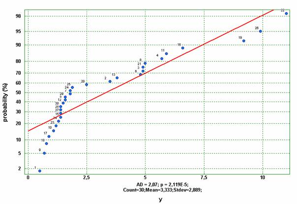
Probability of observations as function of the particle’s size under normality assumption.