Analysis of Variance - ANOVA
QstatLab can be used to perform single-factor or multi-factor analysis of variance. This will be shown with an example that studies the strength (y) of three type of cement. For each type (k = 3) we have 6 observations (r = 6). The data are shown in the table below. These data are store in file 9-ANOVA.qsl in columns B and y.
Click the ANOVA button tool to select entered data and produce ANOVA analysis.
The results from ANOVA are shown on the following textual screen. It is possible to choose different type of analysis and diagrams by using the dropdown menu on the right.
It is possible to add several diagrams on the same screen. Use the 'Add plot' button to add a plot, then click on the plot itself to activate it (turns blue) and then change the type of the plot as above.
The following screenshot shows a collection of several plots of different types
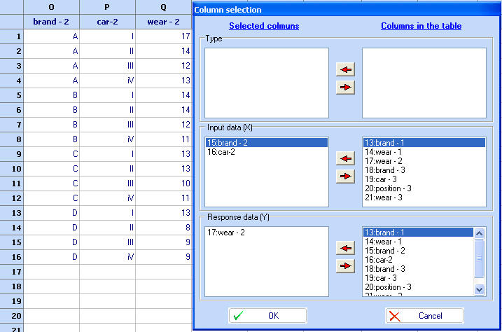
Another example shows multi-factor ANOVA. It studies the wear (wear-2) of various brands (brand-2) of tyres and cars (car-2).
If there are repeated observations, the residual sum has two components - Residual1 (represents the errors between the groups of data - the scatter of the factor levels) and Residual2 (represents the errors inside the groups of data (the scatter of data for equal factor levels). We can illustrate this with the following example, where inputs are columns X1, X2, X3, X4 and response data is Y. Part of the ANOVA results is as follows:
Source
Sums DF Variance
F P
x1
26673.39372 1 26673.39372 6.70813 0.00989
x2
11524.46680 1 11524.46680 2.89831 0.08933
x3
14379.73837 1 14379.73837 3.61638 0.05782
x4
727137.69045 1 727137.69045 182.86900 0.00000
Residual11 11432.64199 11 10130.24018
Residual21 777298.63875 464 3830.38500
Residual1 888731.28074 475 3976.27638
-------------------------------------------------------------------------
Total 2668446.57009 479
Pooled Stdev = 63.05772 R-sq = 0.29220 R-sq (adj) = 0.28624
See also