Friction welding
Sources:
- Barker, T, Clausing D. (1984). Quality engineering by design. The Taguchi method. The International QC forum. 11, No.8,28-52.
- Vuchkov, I.N., Boyadjieva, L.N. (2001). Quality improvement with design of experiments. A response surface approach. Kluwer Academic Publishers, Dordrecht.
Methods:
Spreadsheet calculations, interpolations, Taguchi method, ANOVA, Regression analysis, Analytical models in robust engineering, Optimization, Contour plots, 3D plots.
Files: Friction welding – Loss function 1.qsl, Friction welding – Param design 2.qsl, Friction welding – Verification 3.qsl, Friction welding – Loss function 1.qsl, Friction welding – Tolerance design 4.qsl, Friction welding – Regression 5.qsl, Friction welding – Analytical - 6.qsl.
Short description of the problem:
Barker and Clausing (1984) used
Taguchi method to find a welding system that reduces or prevents shaft breakage
of the propeller in a high powered outboard engine. Performance characteristic y
is the tensile strength. The target is to obtain y approximately equal
to 160, while keeping standard deviation below 20. The factors are listed in
Table 1. Denote by![]() ,
, ![]() the values of
factors measured in a physical scale. Their ranges are
the values of
factors measured in a physical scale. Their ranges are![]() .
.
Barker and Clausing used a crossed
array consisting of an ![]() orthogonal array as a
parameter design matrix (columns 2 to 7 of Table 2) and a
orthogonal array as a
parameter design matrix (columns 2 to 7 of Table 2) and a ![]() orthogonal array as
a noise matrix. The total number of runs is
orthogonal array as
a noise matrix. The total number of runs is ![]() . The variations of the
process parameters within the tolerance limits shown in Table 1 are considered
as noises. The
. The variations of the
process parameters within the tolerance limits shown in Table 1 are considered
as noises. The ![]() orthogonal array is conducted
for each row of the parameter design. The levels of the noise factors in it are
chosen equal to
orthogonal array is conducted
for each row of the parameter design. The levels of the noise factors in it are
chosen equal to ![]() and
and![]() . For example, for
the first run of Table 2 the first parameter is
. For example, for
the first run of Table 2 the first parameter is ![]() which corresponds to
which corresponds to ![]() rpm.
According to Table 2 the low cost tolerance of
rpm.
According to Table 2 the low cost tolerance of ![]() is
is![]() . Therefore, the
levels of
. Therefore, the
levels of ![]() in the
in the ![]() array for the first
run of Table 2 are 900, 1000 and 1100 rpm.
array for the first
run of Table 2 are 900, 1000 and 1100 rpm.
TABLE 1. Factor levels, low cost tolerances and half
ranges of factor variations for the friction welding example.
|
Factors
|
Speed
(rpm) |
Heating pressure (psi) |
Upset pressure (psi) |
Length
(thous) |
Heating time (sec) |
Upset time (sec) |
|
|
|
|
|
|
|
|
|
1-st level (p = -1) |
1000 |
4000 |
8500 |
-30 |
2.8 |
3.2 |
|
2-nd level (p = 0 ) |
1200 |
4400 |
9000 |
0 |
3.2 |
3.6 |
|
3-rd level (p = 1 ) |
1400 |
4800 |
9500 |
30 |
3.6 |
4.0 |
|
Low cost tolerances
|
|
|
|
|
|
|
|
Half ranges of variation
|
200 |
400 |
500 |
30 |
0.4 |
0.4 |
Barker and Clausing do not display the full crossed array. They give only the parameter design and the tensile strength y, standard deviation of y, and signal-to-noise ratio. They are shown in Table 2. The data of Table 2 are given also in the file Friction welding – Param design.qsl.
TABLE 2. Parameter design, tensile strength, standard deviation and S/N ratio
|
|
SPEED |
HTPRS |
UPPRS |
LENGTH |
HTTIME |
UPTIME |
STRENGTH |
|
|
|
No. |
|
|
|
|
|
|
y |
s |
|
|
1 |
1000 |
4000 |
8500 |
-30 |
2,8 |
3,2 |
104.3 |
38.04 |
34.2 |
|
2 |
1000 |
4000 |
9000 |
0 |
3,2 |
3,6 |
135.1 |
27.89 |
39.9 |
|
3 |
1000 |
4000 |
9500 |
30 |
3,6 |
4 |
128.6 |
45.16 |
12.3 |
|
4 |
1000 |
4400 |
8500 |
0 |
3,2 |
4 |
123.8 |
42.41 |
25.6 |
|
5 |
1000 |
4400 |
9000 |
30 |
3,6 |
3,2 |
134.6 |
45.59 |
37.5 |
|
6 |
1000 |
4400 |
9500 |
-30 |
2,8 |
3,6 |
134.7 |
27.06 |
40.0 |
|
7 |
1000 |
4800 |
8500 |
30 |
3,6 |
3,6 |
150.6 |
38.88 |
40.6 |
|
8 |
1000 |
4800 |
9000 |
-30 |
2,8 |
4 |
116.2 |
43.24 |
28.6 |
|
9 |
1000 |
4800 |
9500 |
0 |
3,2 |
3,2 |
151.2 |
45.03 |
39.7 |
|
10 |
1200 |
4000 |
8500 |
0 |
3,6 |
3,6 |
134.2 |
31.73 |
39.6 |
|
11 |
1200 |
4000 |
9000 |
30 |
2,8 |
4 |
134.1 |
41.28 |
35.4 |
|
12 |
1200 |
4000 |
9500 |
-30 |
3,2 |
3,2 |
132.0 |
40.67 |
39.1 |
|
13 |
1200 |
4400 |
8500 |
30 |
2,8 |
3,2 |
125.8 |
38.47 |
37.9 |
|
14 |
1200 |
4400 |
9000 |
-30 |
3,2 |
3,6 |
140.9 |
28.67 |
40.5 |
|
15 |
1200 |
4400 |
9500 |
0 |
3,6 |
4 |
158.5 |
46.85 |
37.8 |
|
16 |
1200 |
4800 |
8500 |
-30 |
3,2 |
4 |
129.6 |
44.86 |
30.9 |
|
17 |
1200 |
4800 |
9000 |
0 |
3,6 |
3,2 |
164.5 |
50.00 |
41.3 |
|
18 |
1200 |
4800 |
9500 |
30 |
2,8 |
3,6 |
156.1 |
29.91 |
41.7 |
|
19 |
1400 |
4000 |
8500 |
30 |
3,2 |
4 |
111.7 |
43.96 |
12.5 |
|
20 |
1400 |
4000 |
9000 |
-30 |
3,6 |
3,2 |
109.6 |
46.74 |
31.1 |
|
21 |
1400 |
4000 |
9500 |
0 |
2,8 |
3,6 |
146.7 |
30.60 |
40.8 |
|
22 |
1400 |
4400 |
8500 |
-30 |
3,6 |
3,6 |
125.6 |
37.59 |
38.3 |
|
23 |
1400 |
4400 |
9000 |
0 |
2,8 |
4 |
128.3 |
44.40 |
34.6 |
|
24 |
1400 |
4400 |
9500 |
30 |
3,2 |
3,2 |
139.1 |
44.84 |
39.3 |
|
25 |
1400 |
4800 |
8500 |
0 |
2,8 |
3,2 |
119.9 |
44.07 |
35.2 |
|
26 |
1400 |
4800 |
9000 |
30 |
3,2 |
3,6 |
148.0 |
36.84 |
40.8 |
|
27 |
1400 |
4800 |
9500 |
-30 |
3,6 |
4 |
150.1 |
53.13 |
34.1 |
A fragment of QSTATLAB spreadsheet for this example is shown below

- Data analysis by Taguchi method (Barker & Clausing)
Loss function:
Barker & Clausing calculated Taguchi’s loss function :
![]() ,
,
where ![]() is the target value for the
strength. They estimated that a reduction of tensile strength by 60 incurs a
loss of $ 500. Putting these values in L they obtained:
is the target value for the
strength. They estimated that a reduction of tensile strength by 60 incurs a
loss of $ 500. Putting these values in L they obtained:
![]() . Therefore:
. Therefore:
![]()
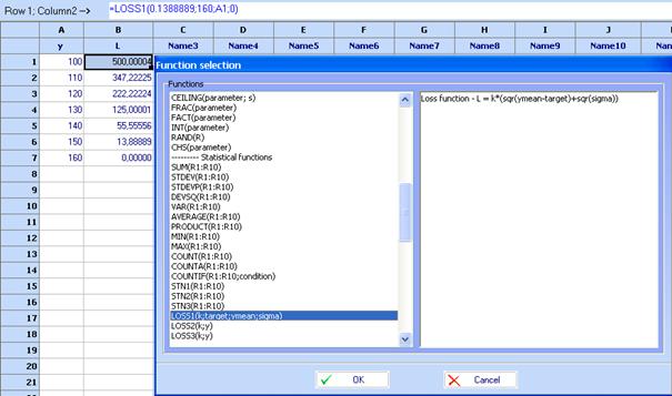
Let us calculate the loss function for strength values from 100 to 160, step 10. QstatLab has built-in functions for Taguchi’s loss functions. A function called LOSS1(k; target; ymean; sigma) calculates the following loss function:
![]() .
.
We can use it to calculate ![]() putting k
= 0.1388889, target = 160, ymean =A1 and sigma = 0.
putting k
= 0.1388889, target = 160, ymean =A1 and sigma = 0.
Click ![]() and select LOSS1(k; target; ymean;
sigma) and enter the above values for variables in the brackets. The value in
cell B1 is 500.0004. Drag downward the point in the right bottom corner of cell
B1 to obtain the other values of the loss function. The results are shown in
column B of the spreadsheet below.
and select LOSS1(k; target; ymean;
sigma) and enter the above values for variables in the brackets. The value in
cell B1 is 500.0004. Drag downward the point in the right bottom corner of cell
B1 to obtain the other values of the loss function. The results are shown in
column B of the spreadsheet below.
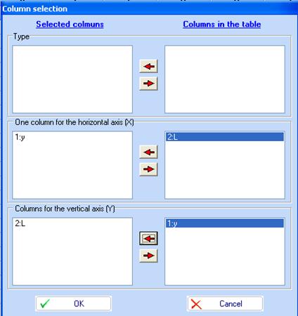
We can plot the loss function using “Interpolations”
of QstatLab (![]() ).
Select the columns as shown below:
).
Select the columns as shown below:
Click OK to obtain the following diagram:
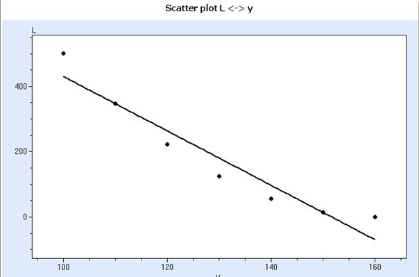
QSTATLAB uses by default linear regression for approximation of the data. It is clear that the linear approximation does not fit the data well enough. That is why click “Options → Diagram → Interpolation (L) → Type linear – y = a+bx” to open the following window:
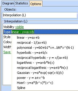
Select polynomial – y =b0+b1*x+…+bN*x^(N-1) and then choose “Polynomial order(L) = 2”:
![]()
Following plot will be obtained:
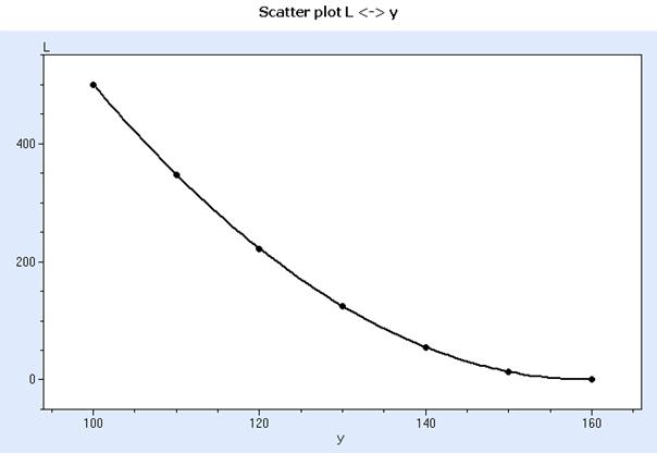
The statistical analysis shows very good approximation, which was expected:
General information for the data set y -L
-------------------------------------------------------------
Designated as X is y
Designated as Y is L
Number of elements:7
Average for X = 130,0000
Average for Y = 180,5556
Qx = 2800,0000
Qy = 210648,1819
Qxy = -23333,3352
Quality of fit = 1,0000
Trend line equation: 3556 -44,44*x+ 0,1389*x^ 2
Statistical analysis and selection of parameter values by use of ANOVA:
Taguchi method makes conclusions on
the basis of ANOVA results for mean values and signal-to-noise ratios. Consider
first ANOVA for the tensile strength (file: Friction welding – Param design 2.qsl).
Click ![]() icon
and select factors and tensile strength as is shown below:
icon
and select factors and tensile strength as is shown below:
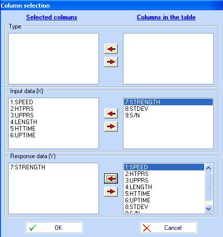
Click OK to obtain following ANOVA table:
Analysis of Variance (ANOVA) for STRENGTH - (SPEED; HTPRS; UPPRS; LENGTH; HTTIME; UPTIME)
-------------------------------------------------------------------------
Name Name Levels Levels
x1 SPEED 3 1000; 1200; 1400
x2 HTPRS 3 4000; 4400; 4800
x3 UPPRS 3 8500; 9000; 9500
x4 LENGTH 3 -30; 0; 30
x5 HTTIME 3 2,8; 3,2; 3,6
x6 UPTIME 3 3,2; 3,6; 4
-------------------------------------------------------------------------
Source Sums DF Variance F P
x1 691,94296 2 345,97148 7,91359 0,00502
x2 1248,33407 2 624,16704 14,27691 0,00042
x3 1634,01407 2 817,00704 18,68785 0,00011
x4 839,44296 2 419,72148 9,60052 0,00237
x5 452,00519 2 226,00259 5,16948 0,02083
x6 612,73407 2 306,36704 7,00770 0,00778
Residual 612,06074 14 43,71862
-------------------------------------------------------------------------
Total 6090,53407 26
Pooled Stdev = 6,61201 R-sq = 0,89951 R-sq (adj) = 0,81337
Confidence intervals for the mean, for each level
Confidence intervals are calculated on the basis of the standard deviation
for each factor level
Level Count Mean Variance 95% Confidence interval
SPEED
1000 9 131,01111 228,14861 119,4007 <= 131,0111 <= 142,6215
1200 9 141,74444 202,17278 130,8149 <= 141,7444 <= 152,6739
1400 9 131,00000 244,50250 118,9807 <= 131,0000 <= 143,0193
HTPRS
4000 9 126,25556 203,83278 115,2813 <= 126,2556 <= 137,2298
4400 9 134,58889 118,24111 126,2305 <= 134,5889 <= 142,9473
4800 9 142,91111 283,20111 129,9755 <= 142,9111 <= 155,8467
UPPRS
8500 9 125,05556 174,37028 114,9053 <= 125,0556 <= 135,2058
9000 9 134,58889 264,62611 122,0847 <= 134,5889 <= 147,0931
9500 9 144,11111 118,06861 135,7588 <= 144,1111 <= 152,4634
LENGTH
-30 9 127,00000 219,31500 115,6166 <= 127,0000 <= 138,3834
0 9 140,24444 246,66028 128,1722 <= 140,2444 <= 152,3167
30 9 136,51111 190,41111 125,9043 <= 136,5111 <= 147,1179
HTTIME
2,8 9 129,56667 246,34750 117,5021 <= 129,5667 <= 141,6313
3,2 9 134,60000 148,51500 125,2325 <= 134,6000 <= 143,9675
3,6 9 139,58889 309,95361 126,0561 <= 139,5889 <= 153,1217
UPTIME
3,2 9 131,22222 366,31444 116,5104 <= 131,2222 <= 145,9340
3,6 9 141,32222 94,82944 133,8369 <= 141,3222 <= 148,8075
4 9 131,21111 223,58111 119,7175 <= 131,2111 <= 142,7047
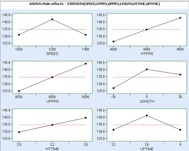
Main effects plots for tensile strength are shown below. The results of this analysis show that all factors are significant at significance level 0.05.
Consider now ANOVA results for S/N ratio. The corresponding ANOVA table is:
Analysis of Variance (ANOVA) for S/N - (SPEED; HTPRS; UPPRS; LENGTH; HTTIME; UPTIME)
-------------------------------------------------------------------------
Name Name Levels Levels
x1 SPEED 3 1000; 1200; 1400
x2 HTPRS 3 4000; 4400; 4800
x3 UPPRS 3 8500; 9000; 9500
x4 LENGTH 3 -30; 0; 30
x5 HTTIME 3 2,8; 3,2; 3,6
x6 UPTIME 3 3,2; 3,6; 4
-------------------------------------------------------------------------
Source Sums DF Variance F P
x1 132,32519 2 66,16259 2,68054 0,10337
x2 165,83407 2 82,91704 3,35933 0,06432
x3 79,33407 2 39,66704 1,60709 0,23534
x4 74,03630 2 37,01815 1,49977 0,25694
x5 24,89407 2 12,44704 0,50428 0,61450
x6 736,44519 2 368,22259 14,91831 0,00034
Residual 345,55630 14 24,68259
-------------------------------------------------------------------------
Total 1558,42519 26
Pooled Stdev = 4,96816 R-sq = 0,77827 R-sq (adj) = 0,58821
Confidence intervals for the mean, for each level
Confidence intervals are calculated on the basis of the standard deviation
for each factor level
Level Count Mean Variance 95% Confidence interval
SPEED
1000 9 33,15556 90,41778 25,8464 <= 33,1556 <= 40,4647
1200 9 38,24444 11,41028 35,6480 <= 38,2444 <= 40,8409
1400 9 34,07778 76,43444 27,3576 <= 34,0778 <= 40,7980
HTPRS
4000 9 31,65556 129,06278 22,9230 <= 31,6556 <= 40,3881
4400 9 36,83333 20,67500 33,3382 <= 36,8333 <= 40,3284
4800 9 36,98889 24,33611 33,1969 <= 36,9889 <= 40,7809
UPPRS
8500 9 32,75556 79,82278 25,8880 <= 32,7556 <= 39,6231
9000 9 36,63333 20,79000 33,1285 <= 36,6333 <= 40,1382
9500 9 36,08889 84,27361 29,0325 <= 36,0889 <= 43,1453
LENGTH
-30 9 35,20000 19,62750 31,7946 <= 35,2000 <= 38,6054
0 9 37,16667 24,34250 33,3742 <= 37,1667 <= 40,9591
30 9 33,11111 141,57861 23,9650 <= 33,1111 <= 42,2572
HTTIME
2,8 9 36,48889 16,74361 33,3436 <= 36,4889 <= 39,6342
3,2 9 34,25556 93,96528 26,8044 <= 34,2556 <= 41,7067
3,6 9 34,73333 80,98250 27,8161 <= 34,7333 <= 41,6506
UPTIME
3,2 9 37,25556 10,23028 34,7970 <= 37,2556 <= 39,7141
3,6 9 40,24444 0,91278 39,5101 <= 40,2444 <= 40,9788
4 9 27,97778 91,60444 20,6208 <= 27,9778 <= 35,3347
ANOVA table shows that significant effects for the S/N ratio are UPTIME at significance level 0.05, SPEED and HTPRS at significance level 0.1. The corresponding main effects plots are shown below:
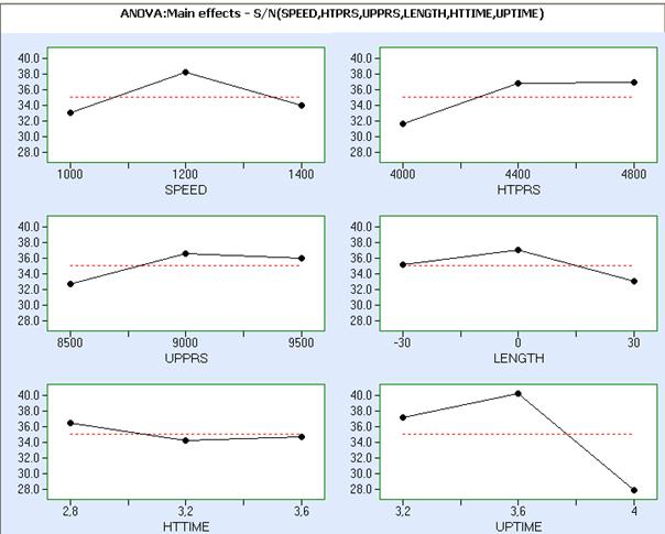
Barker & Clausing make following conclusions based on main effects graphs for the tensile strength and S/N ratio:
“Our analysis has shown that three of the factors have a significant effect on the S/N (“control”), while the other three only significantly effect the mean (”signal”) level. This is an advantage, since we can use the control factors to hold the variation to a proper level and move the mean with the signal factors. Our plots show us where to set the parameters. Speed is best at its mid-point of 1200 RPM. Heat pressure is best at 4800 psi. Upset pressure is a signal factor and is set to maximize the average strength at 9500 psi. Length is best at zero deviations from nominal. Heat time gives the highest signal at 3.6 sec, even though the S/N is best at 2.8. Since this factor does not exhibit a statistically significant effect for S/N we move the level in favor of the mean response. The upset time is best set at the 3.6 or midpoint level.”
Tolerance design:
Barker & Clausing have performed a L18 tolerance design to verify the results obtained through parameter design analysis. In this design they use the optimal values found by parameter design and introducing noises according to the low cost tolerances, given in Table 1 (Friction welding – Verification 2.qsl):
SPEED: 1200 ![]() 10%
10%
HTPRS: 4800 ![]() 15%
15%
UPPRS: 9500 ![]() 15%
15%
LENGTH: 0 ![]() 10%
10%
HTTIME: 3.6 ![]() 20%
20%
UPTIME: 3.6 ![]() 20%
20%
The data are shown below:
We calculate the signal-to-noise ratio using the built-in formula STN3(G1:G18). The formula for S/N ratio is:
 .
.
The S/N ratio is 43.25. We also calculate the standard deviation by the formula: =STDEV(G1:G18). The result is STDEV = 40.15256. Vuchkov & Boyadjieva (2001) showed that this value is biased and the true value is about 50.
The average of the tensile
strength in the verification experiment is calculated by the formula: =AVERAGE(G1:G18).
The result is: ![]() 159,73105. The average
strength is close to the desired, but the standard deviation is still too
large. The loss is still too large:
159,73105. The average
strength is close to the desired, but the standard deviation is still too
large. The loss is still too large: ![]() . In order to decrease the loss
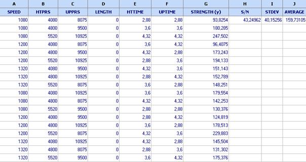
Barker & Clausing decrease the tolerances. They first calculate
contributions of factors on the basis of ANOVA table of L18 noise array (file: Friction
welding – Verification 3.qsl):
. In order to decrease the loss
Barker & Clausing decrease the tolerances. They first calculate
contributions of factors on the basis of ANOVA table of L18 noise array (file: Friction
welding – Verification 3.qsl):
Analysis of Variance (ANOVA) for STRENGTH (y) - (SPEED; HTPRS; UPPRS; HTTIME; UPTIME)
-------------------------------------------------------------------------
Name Name Levels Levels
x1 SPEED 3 1080; 1200; 1320
x2 HTPRS 3 4080; 4800; 5520
x3 UPPRS 3 10925; 8075; 9500
x4 HTTIME 3 2.88; 3.6; 4.32
x5 UPTIME 3 2.88; 3.6; 4.32
-------------------------------------------------------------------------
Source Sums DF Variance F P
x1 774,44053 2 387,22027 1,01216 0,41105
x2 9311,26356 2 4655,63178 12,16938 0,00527
x3 5598,36737 2 2799,18368 7,31680 0,01927
x4 5732,72390 2 2866,36195 7,49240 0,01821
x5 3313,09952 2 1656,54976 4,33006 0,05971
Residual 2677,98530 7 382,56933
-------------------------------------------------------------------------
Total 27407,88018 17
Pooled Stdev = 19,55938 R-sq = 0,90229 R-sq (adj) = 0,76271
An approximate calculation of contributions is based on the sums of squares in ANOVA table and is shown below.
|
SOURCE |
Sum of squares |
% contributions |
|
SPEED |
774.44 |
2.8 |
|
HEAT PRESSURE |
9311.26 |
33.97 |
|
UPSET PRESSURE |
5598.36 |
20.43 |
|
LENGTH |
- |
- |
|
HEAT TIME |
5732.72 |
20.92 |
|
UPSET TIME |
3313.10 |
12.09 |
|
RESIDUAL |
2677.98 |
9.77 |
|
TOTAL |
27407.88 |
|
For example the contribution of the heat pressure to variability is:
![]()
Using this information they decided to decrease the tolerances of the factors as follows:
SPEED: 1200 ![]() 10% (no change)
10% (no change)
HTPRS: 4800 ![]() 5 % (1/3 of the
original)
5 % (1/3 of the
original)
UPPRS: 9500 ![]() 7.5 % (1/2 of the
original)
7.5 % (1/2 of the
original)
LENGTH: 0 ![]() 10 % (no change)
10 % (no change)
HTTIME: 3.6![]() 5 % (1/4 of the
original)
5 % (1/4 of the
original)
UPTIME: 3.6![]() 5 % (1/4 of the
original)
5 % (1/4 of the
original)
A new L18 design was carried out by Barker & Clausing to check the situation after the tolerance shrinking. The design is shown in the Table below (file: Friction welding – Tolerance design – 4)
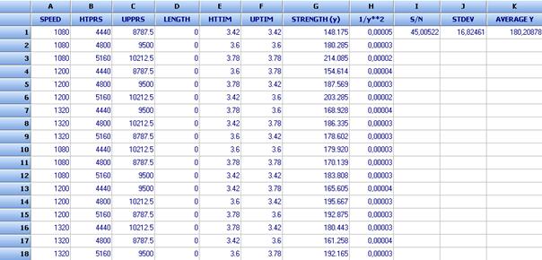
The calculation of S/N ratio, standard deviation and Average (y) has been done by use of the formulae given for the verification experiment.
One can see that after the tolerance design the standard deviation was reduced to 16.82 (before tolerance design it was 40.15). The average strength was increased to 180.21 (before 159.53).
Barker & Clausing reported average loss reduction from $ 350/engine to $ 22/engine. For 10000 engines this makes more than $ 3 million savings.
Conclusions:
- The experiment performed by Barker & Clausing made it possible to improve tensile strength to 180 and to decrease the standard deviation to 16.82.
- As a result the loss was decreased that made more than $ 3 million savings.
- To get these results Barker and Clausing have performed a parameter design with 27x18 = 486 runs, a verification experiment with 18 runs and a tolerance design with 18 runs. The total number of runs was 522.
- The optimal parameter values were found approximately, because in Taguchi method they are selected only amongst the parameter levels in the experiment.
- Model-based approach to friction welding data
A model based approach to the same problem is possible (Vuchkov, Boyadjieva (2001). It reduces drastically the number of experiments and makes more reliable conclusions for the process than Taguchi method.
The model-based approach includes following steps:
- Development of a regression model
- Deriving analytically models of mean value and variance of the performance characteristic
- Minimization of variance while keeping the mean value on target, or minimization of loss function.
In the case of friction welding example we will use only 27 of 522 experiments to get the solution. The reduction of experiments is almost 20 times!
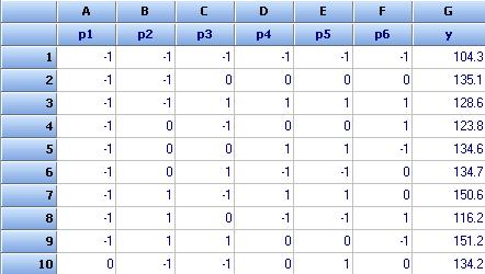
Building a regression model
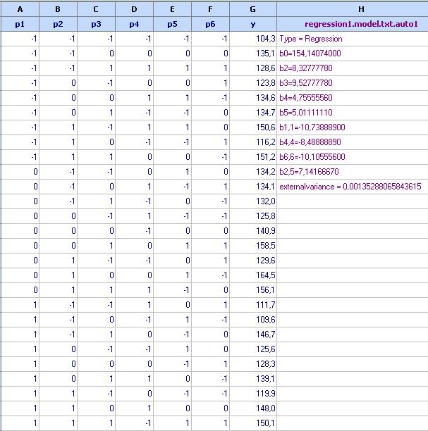
First we rewrite the parameter design in coded form (file: Friction welding – Regression – 5.qsl). Using the command = CODE(A1;1000;1400) and dragging downward we obtain the first column of coded design. The other columns of the parameter design matrix are coded in a similar way. A fragment of this matrix is shown below with the data for tensile strength (y). The full data are in file Friction welding-Regression-5.qsl. It contains also a model obtained at the end of calculations.
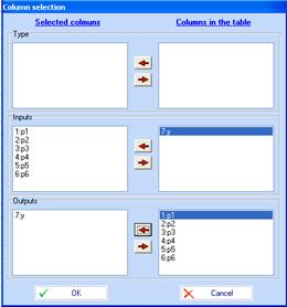
We want to create a second
order regression model for the tensile strength. We will use Regression
analysis (![]() ).We
start with column selection as follows:
).We
start with column selection as follows:
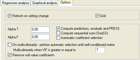
In this example the number of unknown coefficients in a second order polynomial with 6 factors is 28, while the number of runs in parameter design is only 27. That means that information matrix is ill conditioned (there is multicolinearity). Any regression analysis program is unstable under such circumstances. QstatLab can remove some terms so that to avoid multicolinearity. First we check if there are some null value coefficients. To use this option we should set the regression analysis properties as follows:
Click ![]() and select second order
model:
and select second order
model:
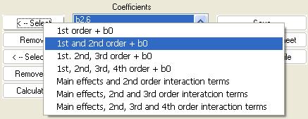
Choosing full second order model we obtain the following:
*** Number of coeffieicnets ( 28) should not be greater than the number of data ( 27)
Results:
*** Ill conditioned matrix (norm: 5200503981,56435) => results might be inaccurate
*** Coefficient b4,6 has a null value and has been excluded from the model.
*** Coefficient b3,6 has a null value and has been excluded from the model.
*** Coefficient b3,5 has a null value and has been excluded from the model.
*** Coefficient b1,5 has a null value and has been excluded from the model.
*** Coefficient b1,2 has a null value and has been excluded from the model.
*** Coefficient b2,6 has a null value and has been excluded from the model.
---------------------------------------------------------------------------
Observations: 27
Input variables: 6
Number of coefficients: 22
Assignments:
x1 <--> p1
x2 <--> p2
x3 <--> p3
x4 <--> p4
x5 <--> p5
x6 <--> p6
y <--> y
---------------------------------------------------------------------------
y = 154.157-0.015x1+8.328x2+9.528x3+4.756x4+5.010x5-0.017x6-10.729x1x1-0.006x2x2+0.006x3x3-8.489x4x4-0.023x5x5
-10.117x6x6+0.002x2x3-0.016x3x4-0.020x4x5-0.011x5x6+0.022x1x3-0.002x1x4+0.020x1x6-0.022x2x4+7.117x2x5
---------------------------------------------------------------------------
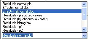
Many of regression
coefficients are close to zero. To select only significant coefficients we click
![]() and select
the Effects half normal plot as follows:
and select
the Effects half normal plot as follows:
The obtained half normal plot of thr effects is:
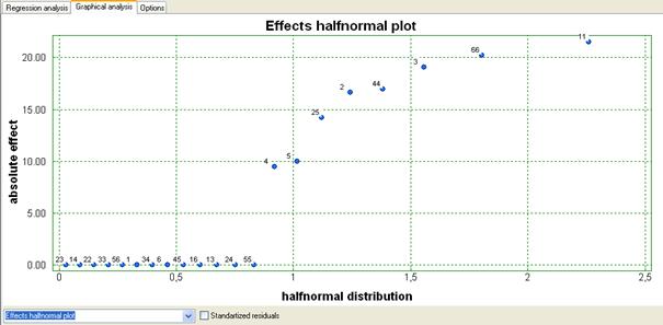
We can delete from the model all terms that are close to zero. Removing all terms with coefficients close to zero we obtain following model:
y = 154.141+8.328x2+9.528x3+4.756x4+5.011x5-10.739x1x1-8.489x4x4-10.106x6x6+7.142x2x5
---------------------------------------------------------------------------
Regressor Coef St. Dev t p Signif VIF
0 154,141 0,019 8230,393 0,000 +
2 8,328 0,009 960,585 0,000 + 1,000
3 9,528 0,009 1099,001 0,000 + 1,000
4 4,756 0,009 548,539 0,000 + 1,000
5 5,011 0,009 578,017 0,000 + 1,000
11 -10,739 0,015 -715,163 0,000 + 1,000
44 -8,489 0,015 -565,323 0,000 + 1,000
66 -10,106 0,015 -672,986 0,000 + 1,000
25 7,142 0,011 672,606 0,000 + 1,000
Significance test was performed at level = 0,05
---------------------------------------------------------------------------
ANOVA
---------------------------------------------------------------------------
Source Sqr. sum DOF Variance F P
Model 6090,50972 8 761,31372 562735,30886 0,00000
Residual 0,02435 18 0,00135
Total 6090,53407 26
--------------------------------------------------------------------------
PRESS
---------------------------------------------------------------------------
N y yp y-yp PRESS(i) SE pred.St. residual
1 104,3000 104,3269 -0,0269 -0,0446 0,0232 -0,9410
2 135,1000 135,0741 0,0259 0,0350 0,0187 0,8190
3 128,6000 128,6324 -0,0324 -0,0538 0,0232 -1,1357
4 123,8000 123,7685 0,0315 0,0395 0,0166 0,9592
5 134,6000 134,5741 0,0259 0,0326 0,0166 0,7899
6 134,7000 134,6741 0,0259 0,0378 0,0206 0,8515
7 150,6000 150,6213 -0,0213 -0,0390 0,0248 -0,7834
8 116,2000 116,2269 -0,0269 -0,0408 0,0215 -0,9004
9 151,2000 151,1519 0,0481 0,0650 0,0187 1,5210
10 134,2000 134,1546 0,0454 0,0925 0,0262 1,7608
11 134,1000 134,1046 -0,0046 -0,0077 0,0232 -0,1622
12 132,0000 131,9907 0,0093 0,0135 0,0206 0,3041
13 125,8000 125,7630 0,0370 0,0541 0,0206 1,2165
14 140,9000 140,8963 0,0037 0,0050 0,0187 0,1170
15 R 158,5000 158,5741 -0,0741 -0,1081 0,0206 -2,4329
16 129,6000 129,5907 0,0093 0,0135 0,0206 0,3041
17 164,5000 164,5157 -0,0157 -0,0262 0,0232 -0,5516
18 156,1000 156,1102 -0,0102 -0,0208 0,0262 -0,3953
19 111,7000 111,7074 -0,0074 -0,0100 0,0187 -0,2340
20 109,6000 109,5935 0,0065 0,0099 0,0215 0,2173
21 146,7000 146,7324 -0,0324 -0,0593 0,0248 -1,1921
22 125,6000 125,6407 -0,0407 -0,0595 0,0206 -1,3381
23 128,3000 128,2852 0,0148 0,0186 0,0166 0,4514
24 139,1000 139,0907 0,0093 0,0116 0,0166 0,2821
25 119,9000 119,9435 -0,0435 -0,0723 0,0232 -1,5251
26 148,0000 147,9963 0,0037 0,0050 0,0187 0,1170
27 150,1000 150,0602 0,0398 0,0662 0,0232 1,3953
---------------------------------------------------------------------------
R denote values with large absolute values of the standartised residual (>2)
---------------------------------------------------------------------------
T(0,025,18)=2,10092; F(0,050,8,18)=2,51016
Residual StDev=0,03678; R-sq=1,00000; Radj-sq=0,99999
PRESS = 0,05967; R-sq(pred)=0,99999
This model is quite good. All correlation coefficients are equal to 1 with 18 degrees of freedom for the residual variance. We can click “Copy to spreadsheet” to save the model in the spreadsheet:
We will work in natural parameter values. That is why we introduce in the regression model all lower and upper levels of the factors. This can be done by use of Model editor. A fragment of these settings in the Model editor is given below:
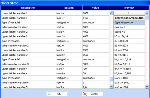
The resulting regression model is:

Deriving mean and variance models with errors in factors
For the model-based approach we need the variance matrix of errors in factors
![]() .
.
This is not given by Barker and
Clausing. We computed estimates of these variances taking into account
Taguchi's recommendation to choose the factor levels in the noise array equal
to ![]() ,
,
![]() and
and
![]() ,
where
,
where ![]() is
the mean value of i-th noise factor,
is
the mean value of i-th noise factor, ![]() is the corresponding standard
deviation,
is the corresponding standard
deviation, ![]() , and
, and ![]() . Therefore, we can
compute an estimate of the noise variance as follows:
. Therefore, we can
compute an estimate of the noise variance as follows:
![]() .
.
The variances of the errors in coded factors can be obtained as follows:
![]() .
.
They depend on ![]() and vary in
the factor space.
and vary in
the factor space.
This special situation can be taken into account with so called range factor for the standard deviation. Here it is
![]()
For most of the cases it is
![]() .
.
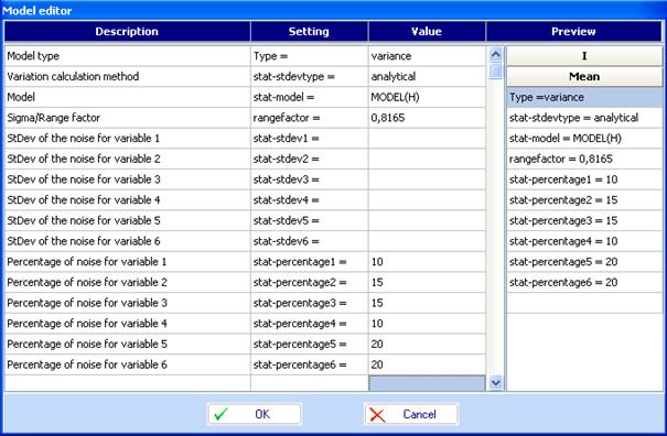
To create a model of the
mean value in the case with errors in factors we use model editor. Click ![]() to call it.
Below is given an example for the model of mean values.
to call it.
Below is given an example for the model of mean values.
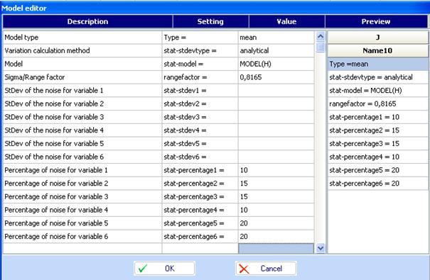
The model is shown in column I of file “Friction welding-Analytical-6.qsl”:
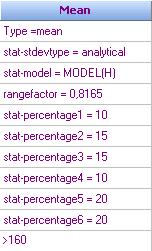
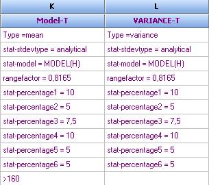
We called the model “Mean” and added an inequality >160, which instructs the program to search values of tensile strength > 160 during the optimization procedure.
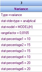
The model of variance is created also by use of model editor:
Click OK to get the following column in the spreadsheet for the variance function:
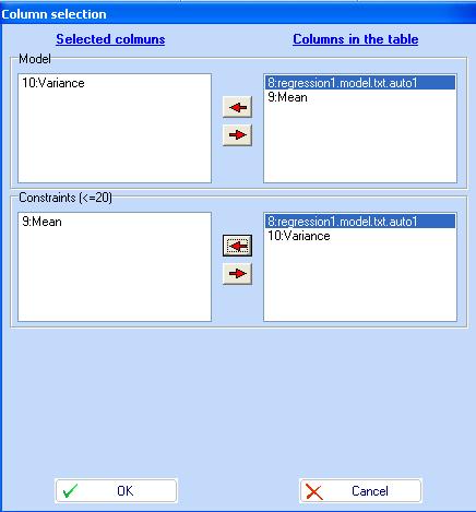
Optimization, contour plots, 3D plots.
With the models defined
above we can do optimization and draw contour plots. A good way to do that is
to use the file: “Friction welding-Analytical-6.qsl” and to click the icon for
contours ![]() .
We consider the Variance as a function to be minimized and the Mean as a
constraint (Mean >160). This can be done by use of the Table for column
selection:
.
We consider the Variance as a function to be minimized and the Mean as a
constraint (Mean >160). This can be done by use of the Table for column
selection:
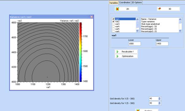
Click OK to start contour drawing. The screen of the computer will look like that:
Click “Optimization” to start optimization procedure. Following will appear:
Click here to open sequences
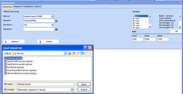
This window defines the starting method (Random search), direction (MIN), Iterations for the initial search (100) and selection of sequence of optimization methods which becomes active after the end of the random search (GAGrad.optseq). The independent variables should be chosen for the search and their initial values too. After selection of a sequence click “Optimize!” to start the procedure.
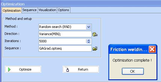
When optimization is completed click “Return”. Following will be seen:
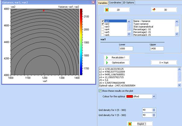
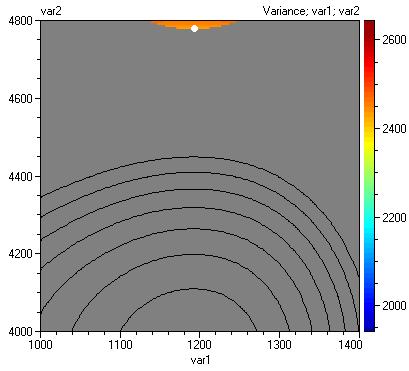
The optimal parameter values are given in the right hand side of the screen. Mark “Show these results on the plot” to get the optimal point. Note however that the plot shown on the figure above does not correspond to optimal factor values. To get a plot for the case when all factors are set on their optimal values click “X = Xopt”. Then following contour plot will be obtained:
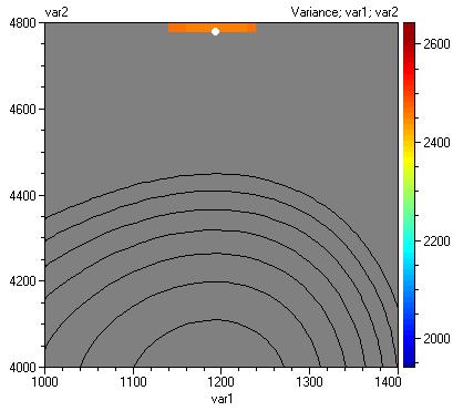
Some refinement of the border can be achieved by increasing grid density for both variables. The Figure above is obtained with grid density 40. If we change it to 100:
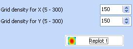
Following contours are obtained:
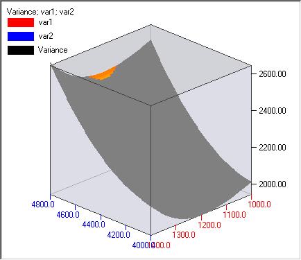
Three dimensional plots are also available. Click “3D” to draw a 3D plot. Then use “3D options” to refine the picture. A 3D plot for the same case is given below.
Tolerance design
A model based tolerance design can also be done. We use the same reduction of tolerances as Barker & Clausing to get comparable results. The tolerances are reduced as follows:
SPEED: 1200 ![]() 10% (no change)
10% (no change)
HTPRS: 4800 ![]() 5 % (1/3 of the
original)
5 % (1/3 of the
original)
UPPRS: 9500 ![]() 7.5 % (1/2 of the
original)
7.5 % (1/2 of the
original)
LENGTH: 0 ![]() 10 % (no change)
10 % (no change)
HTTIME: 3.6![]() 5 % (1/4 of the
original)
5 % (1/4 of the
original)
UPTIME: 3.6![]() 5 % (1/4 of the
original)
5 % (1/4 of the
original)
Using the model editor we define new models, denoted in file: “Friction welding-Analytical-6.qsl” as Mean-T and Variance-T. For example for Mean-T we define following parameters:
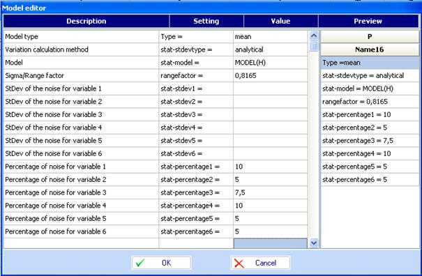
The mean and variance models are defined as follows:
The optimal parameters are now:
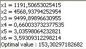
The standard deviation is ![]() , which is
less than the obtained by Barker and Clausing (16.80). The mean strength is 160
as required.
, which is
less than the obtained by Barker and Clausing (16.80). The mean strength is 160
as required.
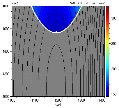
The next figure shows contour plot of Variance-T and Mean-T after tolerance tightening.
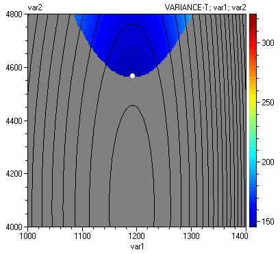
This plot can be additionally refined by putting border on the mean value contour equal to 160 and by changing thickness and colour of the line as follows:
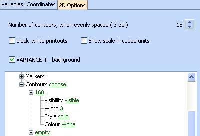
As a result we obtain following plot:
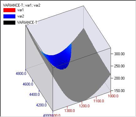
The next figure is a 3D plot:
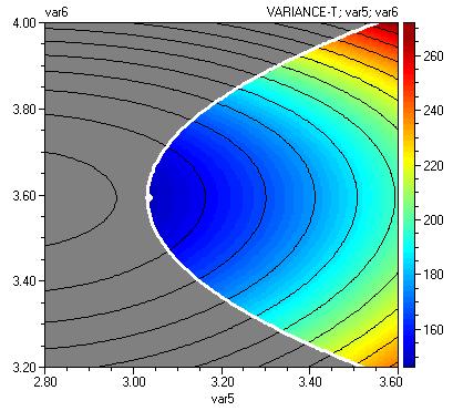
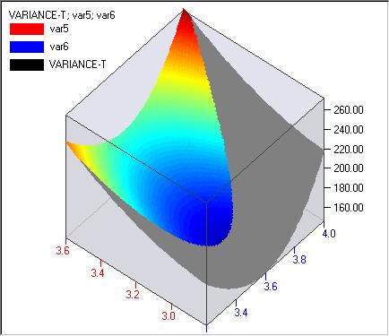
Other contour plots can also be obtained the same way. Contour and 3D plots for p5 and p6 are given below.
Conclusions
- Using model-based approach we obtained results, which are at least as good as the results obtained with Taguchi method. They are better with respect to the variance.
- The number of experiments with the model based approach is about 20 times less than for Taguchi method (Model based approach uses 27 runs, Taguchi method uses 522 runs).
- The model-based approach provides better optimization and graphical procedures.