Dynamic characteristics of parametrically dependent processes
Suppose a design of experiments was used to study a process that depends on several factors х1, х2,..., and for which the measured performance characteristics y changes in time. Such problems exist in pharmaceutical industry when dissolution time of tablets is studied as function of its composition. In rubber industry rheology of a rubber mixture depends on mixture composition. There are similar problems in other industries.
Example. Some property y depends on two factors: х1 and х2. An optimal composite design is carried out and data are measured in 14 equally spaced time intervals and for each combination of factor levels. Standard values are known for each interval (file Stability.qsl in the EXAMPLES folder):
Graphically these data look like that:
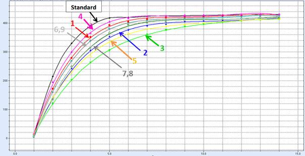
The numbers shown on this plot correspond to the numbers of points in the experimental design. Suppose we need to find such factor combination for which the process is closest to Standard.
Following algorithm is used:
1. Prepare data file as follows (file Stability.qsl):
Important!
The last row (in this example this
is row No. 10)
should contain question
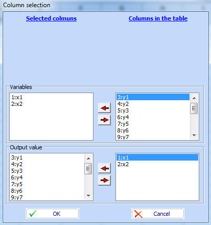
mark (?) instead of factor values. Click icon
![]() and
enter the data as follows:
and
enter the data as follows:
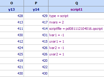
2. Click “OK” and a script model will be created, which is written after the last data column. For our example it looks like that:
QstatLab automatically creates a script model using following algorithm:
1. Create second order regression models for each of time points on the curves (in our example 14 models are created based on data in columns у1,у2,...,у14)
2. Find predicted values for each model and for each point of the experimental design.
3. Find
squared sum of differences between the Standard value (ye) and the predicted
values
in each design point (there are 9 design points for our example, therefore 9
sums of squares are calculated):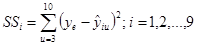
In this expression „i” is the number of design point (i=1,2,…9), and „u“ is model number (u=1,2,3,4,…14)
4.
Find
a regression model, which calculates
![]() as
function of factors
(in
this example х1
and
х2).
This is a script model named “script1”, which
appears in the last column after the data.
as
function of factors
(in
this example х1
and
х2).
This is a script model named “script1”, which
appears in the last column after the data.
5.
Script
model can be used for drawing contour plots or for optimization in a similar
way as any other regression model. Click
![]() and
use model “script1” to plot the following contour diagram:
and
use model “script1” to plot the following contour diagram:
The script model can be used together with models for other performance characteristics in optimization problems. Usually values of factors that provide minimum of squared sum of differences of predicted and observed data are of interest. For our example minimal sum of squares between these values is obtained for х1 = х2 = -1.
The model for deviations of a given curve from the Standard can be used
together with ither regression models for optimization. For example let us
have following model for property Y of the product:
![]()
Suppose that following constraint exists: Y > 50.
A contour plot for this case is given below. The markers on it show
the squared sum of deviations of a given curve from Standard and the white
line shows the constraint for Y.
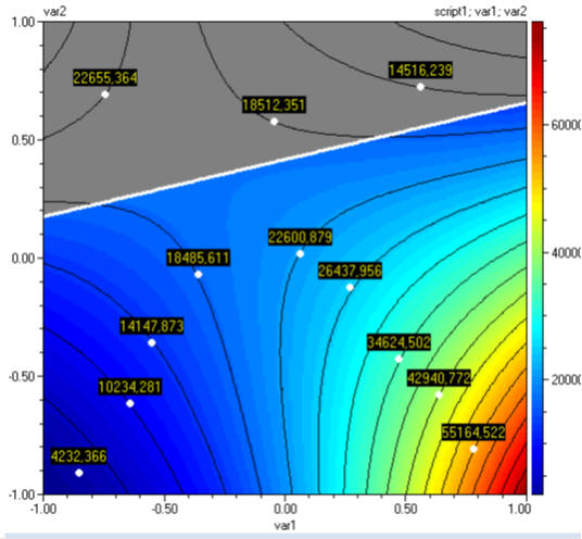
Optimal factor combination is
х1 = х2 = -1.
The grey zone shows combinations of factor for which the constraint Y > 50
does not hold.