Mixtures, linearly dependant variables
- Design of experiment
- Regression analysis
- Ternary plots
- Optimisation
- Mixture experiments analysis with upper- and lower-bounded componentss
- Pseudo-components
Mixtures and linearly independant variables
- Design of experiments
- Selection of designs from "candidate points" using D-Optimality
- Regression analysis, graphical representation, optimisation
Design of Experiments with Mixtures
QstatLab makes it possible to create following designs for mixture experiments:
- Simplex lattices - Scheffe
- Simplex centroid designs - Centroid
- Designs with upper- and lower-bound constraints (known as McLean & Anderson designs or Extreme Vertices designs) - EXTVERT
- Design with random scattered points in the design space – RANDMIX
- Pseudo-components for the case when the constrained region is simplex.
Following option is selected for all types of designs:
![]()
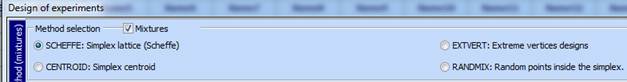
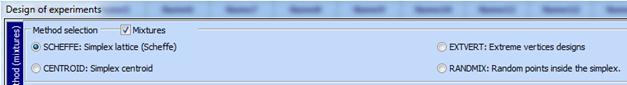
A table for method selection appears and the field “Mixtures” should be selected:
One of the following types of designs can be selected:
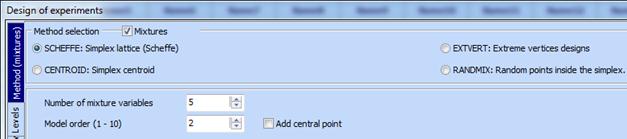
After selection of “Method (mixtures)” mark „SCHEFFE: Simplex lattice (Scheffe)“. The next step is to define the number of mixture components and model order. The table below shows the number of experiments for different combinations of factors’ number and model order.
Number of experiments for different number of linearly dependent factors and model orders (without center point)
|
Factors --> Model order |
3 |
4 |
5 |
6 |
7 |
8 |
9 |
10 |
11 |
12 |
13 |
14 |
15 |
|
1 |
3 |
4 |
5 |
6 |
7 |
8 |
9 |
10 |
11 |
12 |
13 |
14 |
15 |
|
2 |
6 |
10 |
15 |
21 |
28 |
36 |
45 |
55 |
66 |
78 |
91 |
105 |
120 |
|
3 |
10 |
20 |
35 |
56 |
84 |
120 |
165 |
220 |
286 |
364 |
455 |
560 |
680 |
|
4 |
15 |
35 |
70 |
126 |
210 |
330 |
495 |
715 |
991 |
1365 |
|
|
|
|
5 |
21 |
56 |
126 |
252 |
462 |
792 |
1287 |
|
|
|
|
|
|
|
6 |
28 |
84 |
210 |
462 |
924 |
|
|
|
|
|
|
|
|
|
7 |
36 |
120 |
330 |
792 |
|
|
|
|
|
|
|
|
|
|
8 |
45 |
165 |
495 |
1287 |
|
|
|
|
|
|
|
|
|
|
9 |
55 |
220 |
715 |
|
|
|
|
|
|
|
|
|
|
|
10 |
67 |
286 |
1001 |
|
|
|
|
|
|
|
|
|
|
Remarks:
- Adding a center point increases the number of runs by 1
- Table above shows only designs with number of runs no more than approximately 1000. The software can generate designs with more than 1000 runs, but they do not have practical value.
-
If the number of runs is too big it can
be decreased by use of a procedure for D-optimal designs generation and by
choosing a design with desired number of runs
(N
 k).
k).
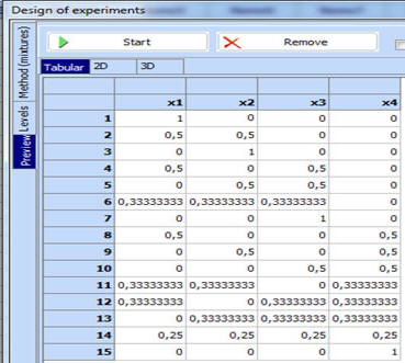
Example. A second order simplex lattice (n = 2) for five mixture components is desired (q=5).
1.
Click
![]() and
select following settings:
and
select following settings:
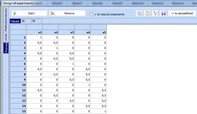
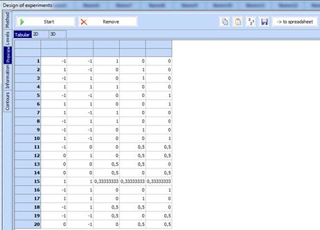
2. Click “Preview” and a table for design building will appear. Then click “Start” and the desired design will be created.
It
can be copied (![]() ),
randomized (
),
randomized (![]() ), saved in a file (
), saved in a file (![]() )
and transferred to spreadsheet (
)
and transferred to spreadsheet (![]() )
)
-
Select
 and
then:
and
then:
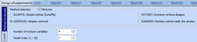
In this type of designs the number of components (linearly dependent variables) is always equal to model order. The number of runs for different number of components is given it the table below.
| Factors |
2 |
3 |
4 |
5 |
6 |
7 |
|
Runs |
3 |
7 |
15 |
31 |
63 |
127 |
- Click “Preview” and then “Start” and the desired design will be created:
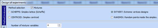
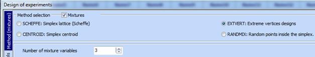
Designs with upper- and lower-bound constraints (Extreme Vertices designs)
-
Select
and
then:
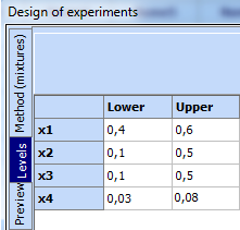
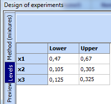
- Click „Levels“ and set constraints:
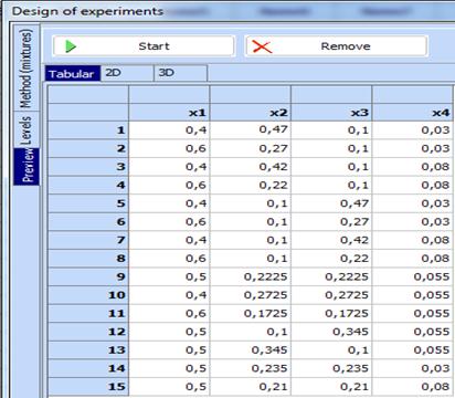
- Click „Preview“, and then „Start“ and the desired design will be created:
Generating random points in the simplex
One can add to a design random points in the simplex space in order to use them as control points. They should conform to the condition:
![]()
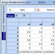
A procedure called RANDMIX: Random points inside the simplex can be used to this end. Let the mixture has 5 components and one wants to generate 7 randomly spread points inside the simplex.
-
Select
and
then
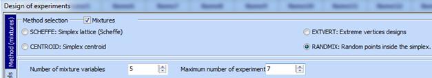
- Click “Preview” and then “Start” and the random points will be generated:
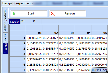
The sum of components in each row is equal to 1.
Regression analysis for experiments with mixtures
Following constraints are imposed on mixture components:
![]() for
for ![]() and
and ![]()
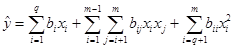
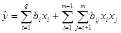
Due to these constraints following changes in the regression analysis procedure are necessary:
Canonical
models should be used. In the canonical models intercept (![]() )
and
second or higher order terms of factors are missing:
)
and
second or higher order terms of factors are missing:
![]()
QstatLab makes it possible to estimate coefficients in linear terms and all interactions up to 4-th order.
· Simplex lattices and simplex centroid designs are saturated designs for which the number of runs is equal to the number of regression coefficients (N=k). That is why only these experiments are not enough for making statistical inference about the regression. Adding new experimental points (“control points”) is recommended, which makes it possible to carry out statistical analysis. The customer can choose them in simplex space taking into account practical considerations. With the control points the number of runs becomes larger than the number of regression coefficients (N>k) and statistical analysis becomes possible. The procedure for regression analysis for simplex lattices and simplex centroid designs is the same.
· Designs for experiments with upper- and lower-bounded constraints (Extreme vertices designs) are usually with more runs than the number of regression coefficients (N>k). This makes unnecessary adding of new “control” points.
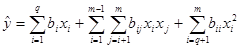
·
When
there are both mixture components (linearly dependent factors) and factors that
vary independently within the interval (-1,1) other type of canonical models
should be used. For example a second order polynomial does not have intercept (![]() ),
squared mixture components and linear terms for independent factors. If the
number of mixture components is q and the number of independent factors is r
(total m = q+r factors) this type of canonical models is:
),
squared mixture components and linear terms for independent factors. If the
number of mixture components is q and the number of independent factors is r
(total m = q+r factors) this type of canonical models is:
Example for regression analysis, drawing contour plots and optimization with simplex lattice design
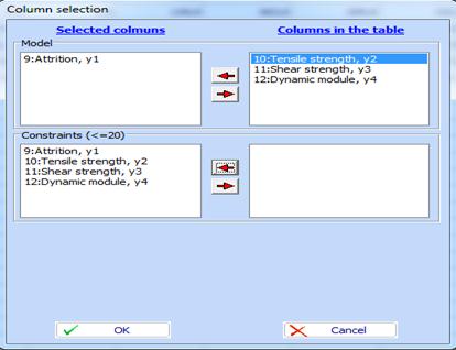
Mixture for heavy conventional tire contains 4 factors (different synthetic rubbers): Rubber 1 ( x1 ), Rubber 2 ( x2 ), Rubber 3 ( x3 ), Rubber 4 ( x4 ). All other components are kept constant. Four tire properties are studied and the constraints for them are as follows:
|
Property |
Y |
Dimension |
Constraint |
|
Attrition resistance |
у1 |
|
>100 |
|
Tensile strength |
у2 |
|
>150 |
|
Shear strength |
у3 |
|
>80 |
|
Dynamic module |
у4 |
|
>80 |
Design of experiments and measured values of the properties for this example are given in a file entitled “Mixtures-heavy tires.qsl”:
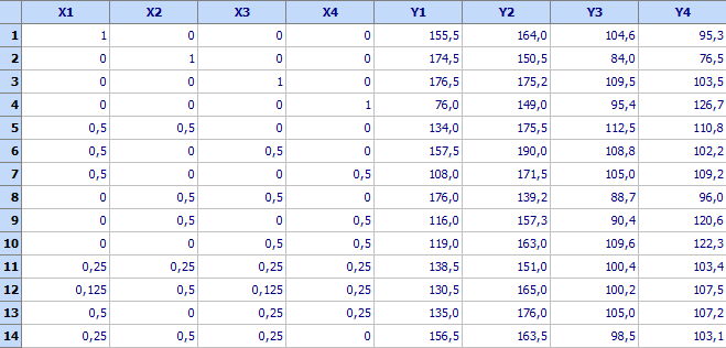
First
10
runs are a simplex lattice and the last 4 are “control
points” added by the customer. To
create a regression model for
у1
click
![]() (Regression
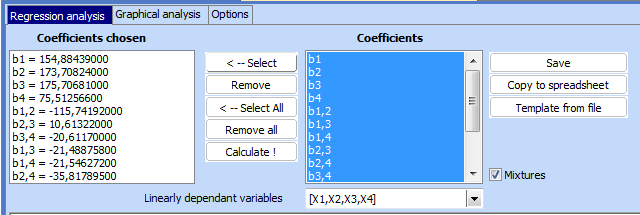
analysis), enter the data and select a model. Mark “Mixtures” in Regression analysis
window and QstatLab will allow appropriate choice of a model for mixture
designs.
(Regression
analysis), enter the data and select a model. Mark “Mixtures” in Regression analysis
window and QstatLab will allow appropriate choice of a model for mixture
designs.
Following results will be obtained:
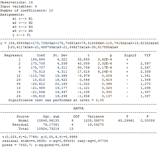
Multiple correlation coefficient is significant (p = 0,00059 < 0,05), but the model has many insignificant coefficients. Delte them one by one starting with coefficients witjh largest value of р. Following model is obtained:
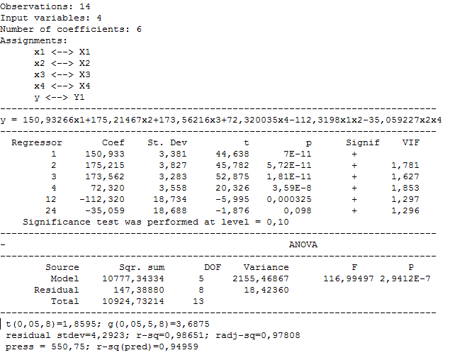
Click
![]() and
the model will be transferred to the spreadsheet.
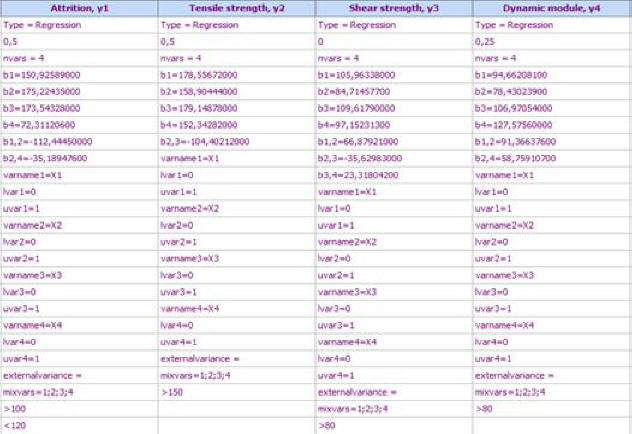
Models for the other properties are obtained
in a similar way. They are:
and
the model will be transferred to the spreadsheet.
Models for the other properties are obtained
in a similar way. They are:
When
the model is transferred to the spreadsheet a row is automatically added:
![]() .
It
shows which are the linearly dependent variables. If there are constraints on
the properties, they are also added at the bottom of the model.
.
It
shows which are the linearly dependent variables. If there are constraints on
the properties, they are also added at the bottom of the model.
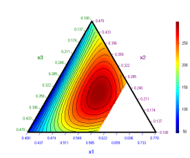
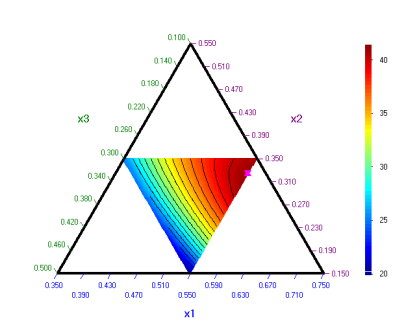
Graphical interpretation (Contour plots)
Regression
models for mixtures can be used to draw contour plots for properties (with or
without constraints). For mixtures the contour plots are triangle diagrams. For
problems with more than 3 components some of them should be set on constant
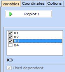
levels. Let us draw a contour plot for y1 with
х1,
х2, х3 on the axes and with x4 = 0. We will also
take into account the constraints imposed on
у1,у2,у3,у4.
Click ![]() and
define the function and the constraints as follows:
and
define the function and the constraints as follows:
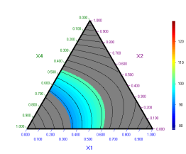
Click “OK” and a contour plot with X4 = 0 will appear. „Приеми“ и се появява диаграма при X4 = 0. All settings are automatically adjusted as follows:
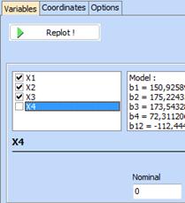
Following doagram will be seen on the desktop:
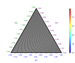
The fact that all the field is grey means that there are not component combinations that conform to all constraints when X4 = 0. Other sections of the surface can be plotted in a similar manner. To this end we should declare the variables on the simplex axes and to set the other factors to some desired values. For example following simpex diagram can be obtained for X3 = 0:
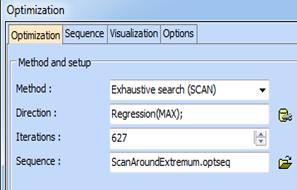
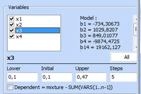
Optimization can help us to get best possible values of components.
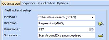
Optimization can be performed as for the case with independent variables. In our example we will look for minimum of the attrition under the constraints defined at the bottom lines of the models. Two optimization methods can be used for mixture problems: exaustive search (scanning) and random search. Following sequence of optimization methods can be also applied: ScanAroundExtremum.optseq.
In
the example we will use scanning and ScanAroundExtremum.optseq. Optimization
program can be activated either from contour plots with double click on ![]() ,
or by a click on following icon:
,
or by a click on following icon: ![]() .
Appropriate settings
should also be selected such as Method, Direction, Number of iterations and
optionally a sequence of optimization algorithms:
.
Appropriate settings
should also be selected such as Method, Direction, Number of iterations and
optionally a sequence of optimization algorithms:
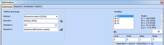
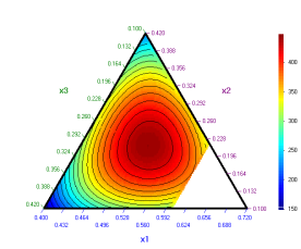
Click “Optimization” and wait for result, then click “Return”. Optimal component’s values will appear near to contour plot:
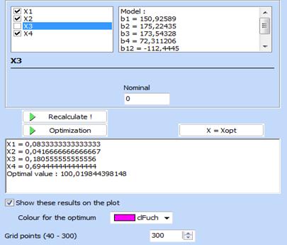
Click X=Xopt and optimal point will be shown on the plot (for х4=0,694) :
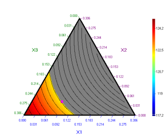
Other sections of the response surface corresponding to other constant values of some of the factors can also be plotted. For example if х3 = 0,1806 following plot is obtained:
Mixture experiments analysis with upper- and lower-bounded components
In this case usually the number of runs is larger than the number of regression coefficients and additional “control points” are not needed. Following should be kept in mind:
- As for the other mixture experiments canonical models should be used (without intercept and second or higher powers of components)
- Constraints are a reason why the simplex space is not fully employed. As a result the contours are plotted only in some part of simplex space.
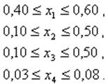
Example (McLean & Anderson (1966)). Consider a railroad flare experiment with objective to maximize the illumination level. The flare consists of four ingredients: magnesium (x1), sodium nitrate (x2), strontium nitrate (x3), and binder (x4). The constraints on the four component proportions were:
A design with lower- and upper- bounded components was used. It is shown together with the measured results in the following table (file Pseudo-McLean.qsl):
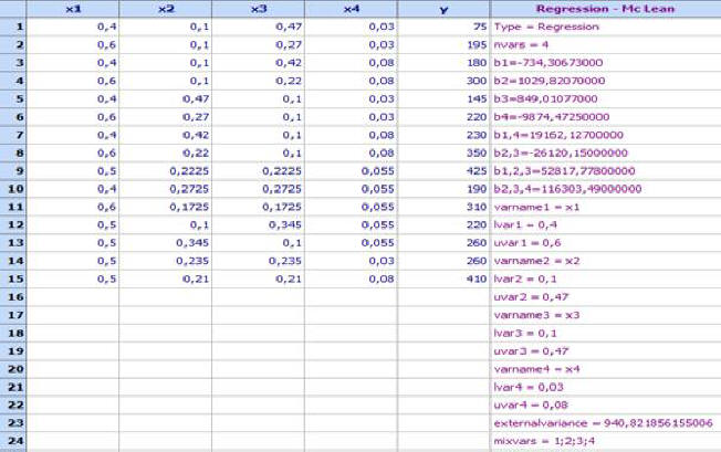
Following regression model has been derived:
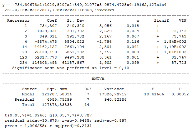
The
model was transferred to the spreadsheet and was used for plotting contours.
The procedure for plotting is the same as for simplex lattices. QstatLab
automatically finds the region in the simplex formed by the constraints on
components. Click icon ![]() .
Select
x3 as “third dependent”. Contour plots for
х1,х2,х3
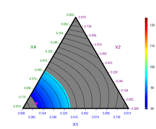
with two different values of x4 are given below.
.
Select
x3 as “third dependent”. Contour plots for
х1,х2,х3
with two different values of x4 are given below.
х4 = 0.03 х4 = 0,08
Optimization problem was defined as follows:
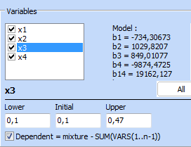
The optimal composition is:
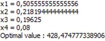
Click X = Xopt to get the optimal point on the contour plot:
This diagram was plotted for х4 = 0.08.
Application of pseudocomponents for constrained simplex space
Pseudocomponents
can be used if the constrained region is simplex. Pseudocomponents are
auxiliary variables for which the constraints typical for a regular simplex
hold (they do not hold for the original components). Denote pseudocomponents as
![]() .
Following constraints are tue for them:
.
Following constraints are tue for them:
![]()
![]()
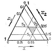
Pseudocomponents are convenient because they make possible to use experimental designs typical for regular simplex, such as Scheffe’s simplex lattices or simplex centroid designs. Below is shown a simplex region with vertices S1,S2,S3, which in original components is arbitrary situated (fig.a). After transformation in pseudocomponents it becomes a regular simplex (fig. b)
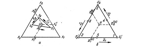
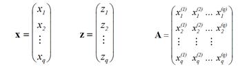
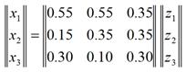
Denote the vertices of the constrained region in original components as follows:
![]()
We can select a design in pseudocomponents and then to rewrite it in original components, so that to make possible it’s use in real experimentation. The transition from pseudocomponents to original ones can be done as follows:
x = Az,
where columns of the matrix А contain coordinates of constrained region vertices:
Example:
Average open time y(s) of a fusible
glue for polygraphy is studied. Following
factors are considered:
![]() -
resin 1,
-
resin 1, ![]() -
resin
2,
-
resin
2, ![]() -
paraffin.
Following constraints are set upon them:
-
paraffin.
Following constraints are set upon them:
![]()
They define following vertices of the constrained region:
![]()
If a simplex lattice in pseudocomponents is used, its coordinates can be transformed to original components by use of equation х = Аz , or:
This can be done by use of QstatLab as follows:
1.
Create a simplex lattice (Scheffe) – icon
![]() and
then:
and
then:
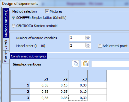
Following has been done to define the problem: a) Option “Mixtures” has been marked, b) simplex lattice (SCHEFFE) has been chosen, c) Number of mixture variables was determined (3), d) model order (2) was set, e) Simplex vertices for the constrained region were defined. Click “Preview” and then “Start” and following experimental design appears:
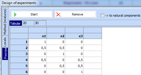
This
design is written in pseudocomponents. It can be transferred to the spreadsheet
using ![]() .
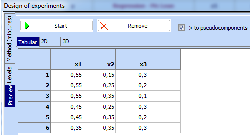
In
order to carry out real experiments it should be
converted
to original components. Mark
the option
.
In
order to carry out real experiments it should be
converted
to original components. Mark
the option ![]() ,
then
the
expression changes to
,
then
the
expression changes to ![]() so
that to be ready for further use. In the same time following design in original
components appears, which can be transferred to the spreadsheet:
so
that to be ready for further use. In the same time following design in original
components appears, which can be transferred to the spreadsheet:
The experiments are carried out and the results are given in the following table:
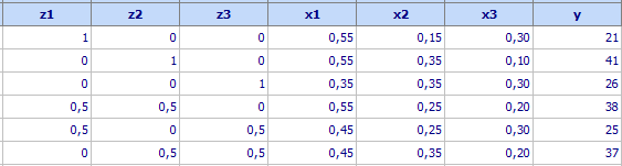
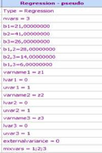
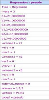
Using Regression analysis for mixtures one can create models both in pseudocomponents and original components. The model in pseudocomponents is:
y = 21z1+41z2+26z3+28z1z2+14z2z3+6z1z3
It is written in QstatLab as shown below:
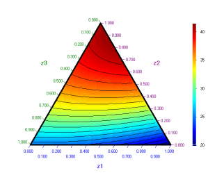
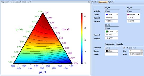
Contour plot in pseudocomponents is:
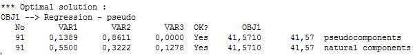
Let us find maximum of the open time y(s) by exhaustive search and using optimization sequence ScanAroundExtremum.optseq. If we want to get the optimal compsition both in pseudo- and original- components we first write in some free cells the coordinates of constrained region vertices. For our exaple these are colums P,Q,R):
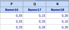
We
also add two last lines on the model for pseudocomponents:
![]() and
and
![]() .
This way we instruct the program that the model was derived in pseudocomponents
and we define the vertices of the restricted sub-simplex. This model is the
following:
.
This way we instruct the program that the model was derived in pseudocomponents
and we define the vertices of the restricted sub-simplex. This model is the
following:
In a graph drawn by use of this model, when we move the cursor on the contour plot the coordinates of the cursor will appear both in pseudocomponents and original components.
The
model can also be used for optimization. Click
![]() and
do the following settings:
and
do the following settings:
The optimal composition is obtained both in pseudocomponents and original (natural) components:
This result can be shown on the plot in pseudocomponents:

Another way for optimization: use a model in original components
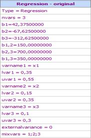
Using Regression analysis a model in original components can be obtained. For our example it is as follows:
y = 42,375x1-67,625x2-312,625x3+150x1x2+700x2x3+350x1x3
In QstatLab it is written as follows:
Click
![]() to
get a contour plot and then click
to
get a contour plot and then click ![]() .
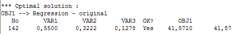
Use
the same settings for the optimization problem as above. Following optimal
solution is obtained:
.
Use
the same settings for the optimization problem as above. Following optimal
solution is obtained:
Mark
![]() to show the optimal point on the contour plot:
to show the optimal point on the contour plot:
The optimal composition is the same as the one obtained by use of pseudocomponents, but the plot is in original components.
Design and analysis of mixture experiments with both mixture components and independent variables
There are two types of factors in this case:
· Mixture components. Suppose that there are q mixture components for which following constraints are true:
![]() ,
i = 1, 2, ..., q (1)
,
i = 1, 2, ..., q (1)
and
 (2)
(2)
Equation (2) means that mixture components are linearly dependent.
· Process variables. They are independent and the condition (2) does not hold for them. Denote the number of independent variables by r. They vary independently within the intervals:
-1![]() 1, (3)
1, (3)
![]()
Let m = q+r is total number of factors.
Models with linearly dependent and independent factors
Following canonical models are used for this problem:
· Linear model with interactions:
 (4)
(4)
Intercept and first order terms are not included in these models, but there are all interactions between linearly dependent and independent factors.
· Second order canonical polynomial:
 (5)
(5)
This model can be obtained from (4) by adding second order terms only for independent variables (there are not second order terms for mixture components).
Design of mixture experiments with linearly dependent and independent factors
Following procedure can be used:
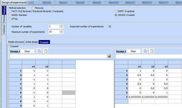
1.
Combine a design for independent factors
(process variables) with some mixture design, for example simplex lattice,
simplex centroid design, extreme vertices design or design in
pseudocomponents. For example of there are three mixture components
![]() and
two independent variables -
and
two independent variables - ![]() the
combined (crossed) design can be graphically presented as follows:
the
combined (crossed) design can be graphically presented as follows:
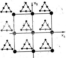
This design will has 6х9 = 54 runs.
2. The number of runs in a crossed design is usually too big. It can be decreased by use of a procedure for D-optimal designs generation. The D-optimal design points are selected amongst the points of the crossed design, also called “candidate points”. The procedure for D-optimal design generation stops when it has implemented a preliminary given number of iterations (equal to the desired number of design points).
When such designs are generated the number of runs N should be larger than the number of coefficients k in a canonical regression model. This will allow statistical analysis of the regression.
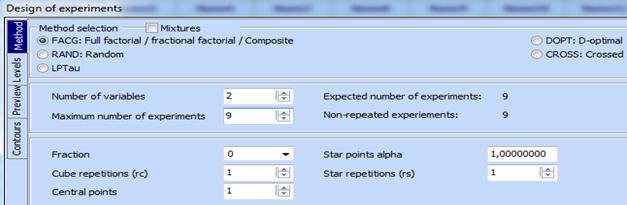
Example. Let us want to generate a second order design for mixture with 3 components (q =3) and two independent factors (r = 2). Use the following procedure:
1.
Click
the icon
![]()
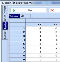
2. Adjust the settings for generation of Optimal composite design for 2 independent variables with 9 points:
3. Click “Preview”, then “Start” and the following design is obtained:
4. Copy this design in the clipboard
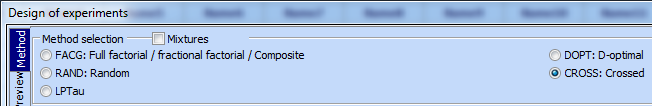
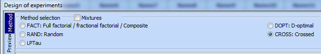
5. Click “Method”, then mark “CROSS:Crossed”
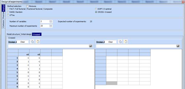
6. Paste from clipboard the design with 2 independent factors in the field named “Design 1”.
7. Mark the field “Mixtures” and then „SCHEFFE: Simplex lattice (Scheffe)“
8. Click “Preview”, then “Start” and generate Scheffe’s second order simplex lattice for 3 components with added central point:
9. Copy the obtained simplex lattice in clipboard
10. Go back to “Method”. A window with marked “CROSS” will appear. Paste the simpex lattice from clipboard to the field “Design 2”:
11. Click “Preview”, then “Start” and a design with 7 х 9 = 63 runs will be obtained. A fragment of this design is shown on the next figure:
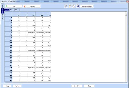
12.
Transfer
the design to the spreadsheed by use of
![]()
In a similar way one can combine any design with independent variables with some mixture design (Simplex lattice, Simplex centroid design, Etreme vertices design (EXTVERT), Random points in the simplex (RANDMIX). The combined designs can be in coded ot natural variables by choice of customer.
Selection of a design with preliminary given “candidate-points” by use of D-optimal design generation procedure
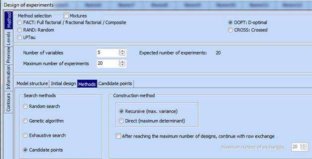
Crossing designs with linearly dependent and independent factors usually produces a design with too big number of runs. It can be decreased by use of D-optimal design generation procedure in which the points are selected from some given “candidate points”
Example. Let three linearly dependent (q = 3), and two independent (r = 2) factors are given. As shown in the previous example the number of runs in a crossed design is 63. A second order canonical model for this problem has 15 coefficients:

For a model with k = 15 coefficients N=63 runs are too much and the experimenter will probably need a design with fewer points. Suppose that the customer wants to generate a 20 runs design. Then N - k = 20 – 15 = 5 degrees of freedom will be available for statistical analysis. To select 20 of 63 points a D-optimal design procedure for selection from given “candidate points” can be used. It runs as follows:
1. Generate a crossed design with 63 points. This was showin in the previous example with q = 3 and r = 2
2. Copy the crossed design with 63 points in the clipboard
3. Go to “Method” and do the following adjustments:
- Mark “DOPT: D-optimal”
- Enter from the keyboard „Number of variables = 5“ and „Maximum number of experiments = 20“
- Click „Methods“ and mark „Candidate-points“
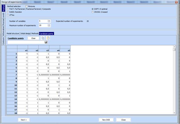
4. Click the key “Candidate points”. A new field called “Candidate points” opens where we should paste from the clipboard preliminary saved crossed design. Mark also the field “DOPT:D-optimal”
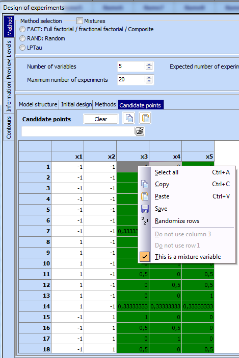
5.
Put
consequtively the cursor on the colums with mixture (linearly dependent)
variables and make a right click to see a menu. Select from the menu the text
![]() .
The colums marked this way will be coloured green and will be considered by the
computer as linearly dependent variables.
.
The colums marked this way will be coloured green and will be considered by the
computer as linearly dependent variables.
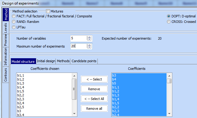
6.
Click
the key
![]() and mark all
coefficients of the desired model in the right field called “Coefficients”. In
our example these are all coefficients in a second order model. They should be
transferred to the left field called “Coefficients chosen” by use of the arrow
and mark all
coefficients of the desired model in the right field called “Coefficients”. In
our example these are all coefficients in a second order model. They should be
transferred to the left field called “Coefficients chosen” by use of the arrow ![]()
7.
Click
“Preview”, then “Start” and a 20 run design will be chosen from 63 candidate
points. This design can be transferred to the spreadsheet by use of the key
![]()
Regression analysis, graphical presentation and optimization for mixtures with linearly dependent and independent factors
Regression analysis and graphical presentation are the same as for the other designs, except for the case of pseudocomponents used in a constrained region. Two examples are given below. In the first one there are not pseudocomponents and in the second transformation to pseudocomponents is used.
Only two methods: exhaustive search and random search can be used for optimization in mixture problems.
Example 1 (without pseudocomponents). Concrete compressive strength on the 28-th day of it’s creation (y, MPa) is studied. Three mixture componets are varied in the experiment. Their sum should always be equal to 1.
|
No |
Component |
Symbol |
Parts of 1 |
|
|
|
|
|
Lower |
Upper |
|
1 |
Crushed sand fraction 0/4 |
Z1 |
0.47 |
0.67 |
|
2 |
Crushed stone fraction 4/16 |
Z2 |
0.105 |
0.305 |
|
3 |
Crushed stone fraction 16/32 |
Z3 |
0.125 |
0.325 |
Value of 1000
kg
is denoted as 1.
The amount of cement
varies independently in the interval from
300
to
400
kg.
We
consider the cement as independent variable, which in coded units is varied in
the interval
![]() and
is set only on its boundary values -1 and 1. There is also water, always in
amount of
200
kg.
As it is constant during the experiment, the water is not
included in the model.
and
is set only on its boundary values -1 and 1. There is also water, always in
amount of
200
kg.
As it is constant during the experiment, the water is not
included in the model.
The problem can be solved in five steps as follows:
- Generate a design for mixture components by use of EXTVERT program
- Create a crossed design
- After receivend results of experiments build a regression model
- Find a composition that provides maximum strength
- Draw contour plots
Let us start with design construction
1.
Click
![]() and
make the following adjustments:
and
make the following adjustments:
2. Set lower and upper bounds
3.
Click “Preview“,
then
„Start“ and
create the design. Randomize it by use of the key
![]() ,
then transfer it to the spreadsheet.
,
then transfer it to the spreadsheet.
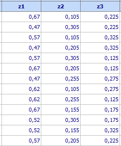
Graphically this design looks like that:
4. In this example crossing consists in repetition of this design twice – once for X4 = -1 and second time for Х4 = 1. Following design is obtained (file Concrete.qsl):
Last coumn contains the measured values of the strength. Call Regression analysis program and do the following adjustments:
5. Select second order model. Following regression model is created:
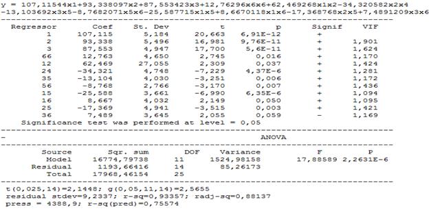
Remove subsequently the coefficients that create strong multicollinearity (too big VIF). They are b13 and then b23. Following model is obtained:
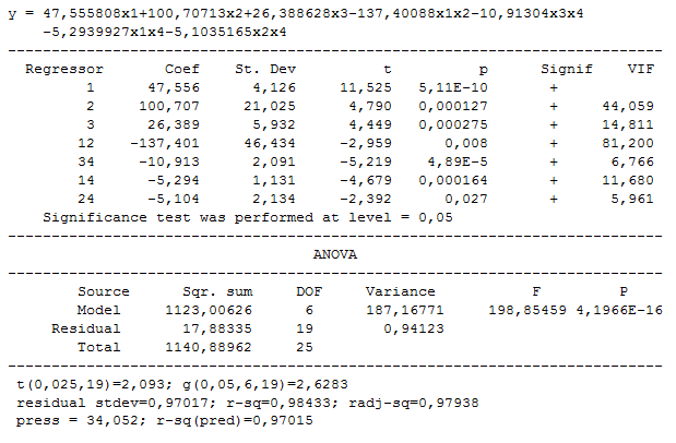
6. Transfer the model to spreadsheet:
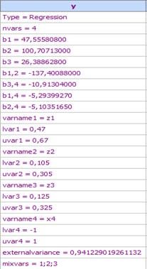
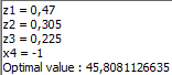
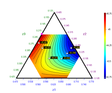
7. Use the model for drawing contour lines and for optimization. The optimal composition is:
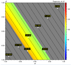
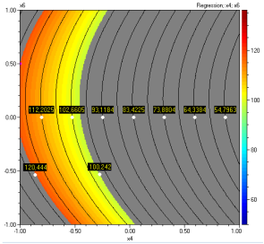
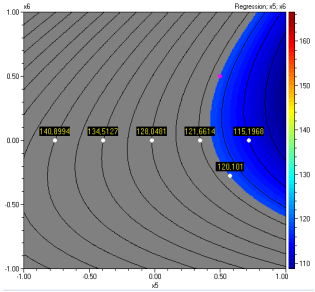
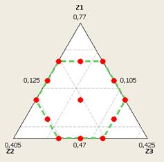
Example 2. (with pseudocomponents). The performance characteristic of interest for a rubber mixture of diaphragm for tires is Modulus at 300 % elongation, y (kg/cm2) The mixtute consists of 3 linearly dependent factors: natural rubber (х1), standard malaysian rubber (х2) and synthetic rubber (х3). Following constraint is imposed so that to make cheaper the composition: х3 > 0,5. In addition there are three independent factors: oil (х4), resin (х5) and accelerator (х6). Following intervals of variation for the independent factors (all measured in weight parts (w.p.)) are set :
|
|
Oil (w.p.) |
Resin (w.p.) |
Accelerator (w.p.) |
|
Basic level (xi = 0) |
3 |
8 |
1,3 |
|
Interval of variation |
3 |
3 |
0,3 |
|
Upper level |
6 |
11 |
1,6 |
|
Lower level |
0 |
5 |
1,0 |
The constraint х3 > 0,5 defines simplex sub-region:
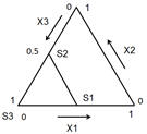
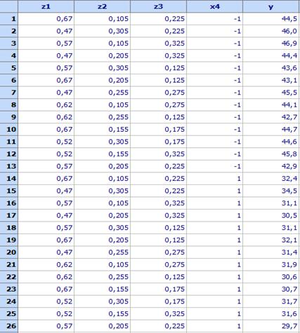
The vertices of the constrained sub-region are with coordinates: S1 (0,5; 0; 0,5), S2 (0; 0,5 ,0,5) and S3 (0; 0; 1). That is why pseudocomponents are used for linearly dependent factors. The design and the measured values of Modulus are given in the file Mixtures-Process variables.qsl and are shown in the following table:
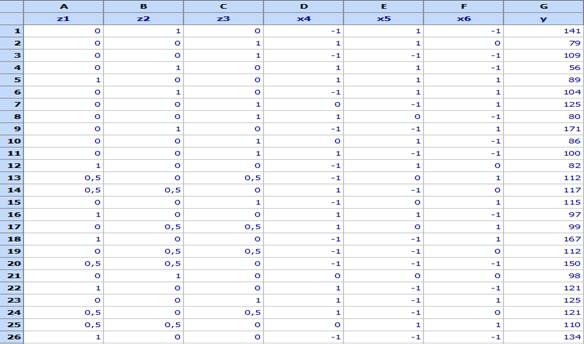
Linearly dependent factors, written in pseudocomponents, are in columns A, B, C. The performance characteristics „Modulus 300 %“(у) is in column G.
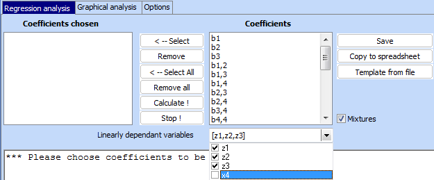
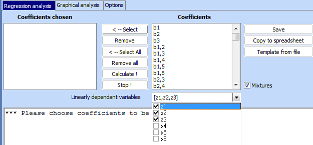
Regression analysis for model in pseudocomponents can be performed as follows:
1.
Select
the icon
![]() and mark the field
“Mixtures”.
Using dropping menu
define the linearly dependent variables:
and mark the field
“Mixtures”.
Using dropping menu
define the linearly dependent variables:
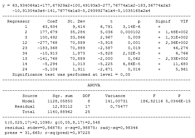
The full model has many insignificant coefficients:
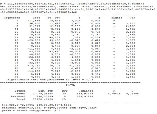
The model can be improved by elimination of insignificant coefficients:
In order to see the results both in coded and in natural variables we should add two more lines in the bottom of the model:
![]()
The model in QstatLab looks like that:
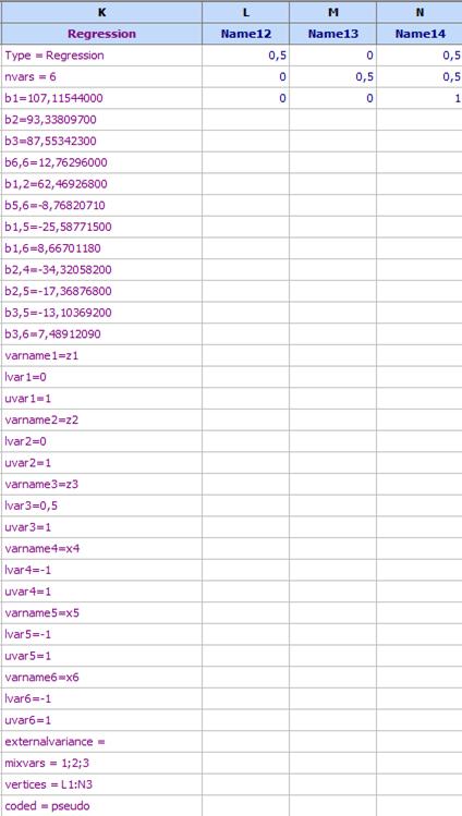
The row “vertices = L1:N3” tells the program that from cell L1 to cell N3 are written the coordinates of vertices of the restricted sub-region. This is used in optimization and in program for drawing contour plots to present the coordinates in natural scale. As a result the plot can be presented in natural scale.
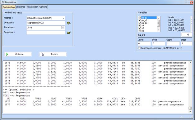
Click “Optimiztion” and do the adjustments shown below. Optimal composition is obtained. The final results of optimization are given in the window below:
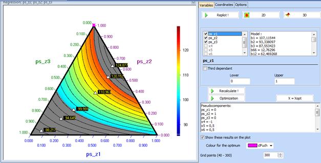
Simplex plot with the optimal composition looks like that:
Contour plots for the independent variables can be drawn
by clicking the key ![]() .
The plots below correspond to optimal values of all variables and are obtained
by clicking the key
.
The plots below correspond to optimal values of all variables and are obtained
by clicking the key
![]()