- Proportions and confidence intervals for proportions
- Example (Contingency.qsl)
- Chi-squared test for two way tables
Proportions and confidence intervals for proportions
Data are sometimes classified in one of two categories: Good/No Good; Pass/Fail; Accepted/Rejected, OK/NOK, etc.
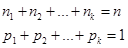
Example 1. Suppose that there are 5 machines in a production line: A,B,C,D and E. A sample of n = 103 defective parts is considered. Fifteen ( n1 = 15 ) defects are produced by machine A, machine B produced n2 = 27 defects, machine C - n3 = 31, machine D - n4 = 19 and machine E - n5 = 11. Denote the corresponding proportions of defective parts as
![]()
If
we could perform infinitly many observations, we would obtain probabilities  of
producing defective parts by the corresponding machines. In
this section we accept following assumptions:
of
producing defective parts by the corresponding machines. In
this section we accept following assumptions:
Probability distribution of proportions is not normal, under the assumptions defined above it is multinomial.
Confidence interval for a proportion can be calculated as follows:
![]()
where
![]() is critical value of standard normal distribution (with
zero mean and variance 1) at significance level
alpha.
For
alpha = 0.05
the
z-value is
is critical value of standard normal distribution (with
zero mean and variance 1) at significance level
alpha.
For
alpha = 0.05
the
z-value is  .
.
Confidence
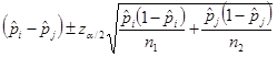
interval for the difference between two proportions  .
It
is calculated as follows:
.
It
is calculated as follows:
Hypothesis test for equality of proportions
The
null hypothesis is: ![]() .
For our example k = 5 and 1/k = 0.2.
.
For our example k = 5 and 1/k = 0.2.
The null hypothesis is accepted if the value 1/k is within confidence intervals for all proportions.
The
null hypothesis: ![]() can
also be tested as follows:
can
also be tested as follows:
- A
value
 is calculated
 - The
null hypothesis is accepted if
 ,
where
,
where 
QstatLab calculates a probability Р. If it is larger than 0.05, the null hypothesis is accepted and if Р < 0.05 the null hypothesis is rejected.
This
algorithm works well enough if 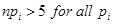
Significance test for difference between two proportions
The
null hypothesis is  .
.
The null hypothesis is accepted if confidence intervals for differences between all pairs of proportions contain zero.
In QstatLab data for Example 1 are written in a row (file: Contingency.qsl)

Click
icon
![]() for Statistics and
following menu will be seen:
for Statistics and
following menu will be seen:
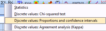
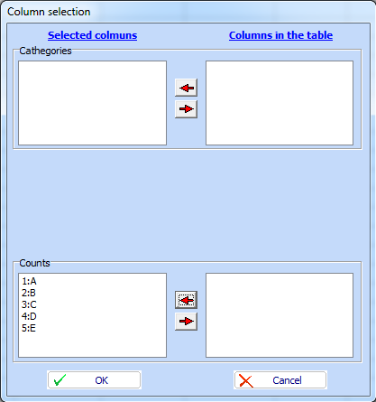
Select “Discrete values: Proportions and confidence intervals”. A menu for column selection will appear. Shift the names of all columns containing information for the problem under consideration from right to left field (Counts):
Click “OK” and a lot of information will appear on the desktop. We will analyze it in three parts.
А) Chi-squared test for proportions
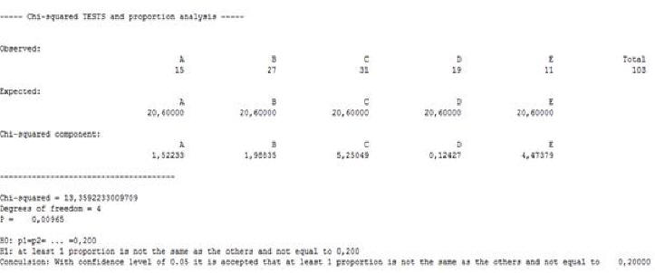
As Р = 0.00965 < 0.05, the null hypothesis for equality of all proportions is rejected. Looking at chi-squared components one can see which proportions differ mostly from value (1/к) = 0.02. The largest component (5.25049) is for machine C. On this machine are obtained much more defective parts (31) than expected (20.6). The next largest component (4.47379) is for machine E. For this machine the observed number of defective parts (11) is much smaller than expected (20.06).
B) Individual confidence intervals
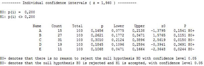
Following notations are used:
· Count is the number of observed defectives for machines A,B,C,D or Е
· The total number of defectives is 103 = 15+27+31+19+11
·
р
is the proportion for
corresponding machine.
For
example for machine А
it
is 0.1456
and is calculated as
15/103.
In the formulae above it is denoted![]() .
.
· „Lower“ and „Upper“ are confidence interval limits.
Hypothesis that all proportions are equal to 0.2 is rejected because the value 0.2 is not within the confidence intervals for C and Е. The proportion of defective parts is larger than 0.2 for machine С and smaller than 0.2 for machine Е.
C) Confidence intervals for difference between two proportions
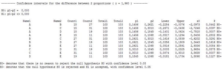
In this problem
„Lower“
and „Upper“
are confidence intervals limits for the difference
between proportions
![]() .
The null hypothesis for equality of proportions is
accepted if zero is within the confidence interval limits. For the example
under consideration the null hypothesis that the differences between all pairs
of proportions are insignificant is rejected. Considerable differences are
observed between following pairs of proportions: А
and B, A and C, B and E, C and D, C and
E.
.
The null hypothesis for equality of proportions is
accepted if zero is within the confidence interval limits. For the example
under consideration the null hypothesis that the differences between all pairs
of proportions are insignificant is rejected. Considerable differences are
observed between following pairs of proportions: А
and B, A and C, B and E, C and D, C and
E.
Chi-squared test for two way tables
This program analyses whether given categorical data depend on two factors. This method can be considered as two-way Analysis of Variance for categorical data.
Example 1. Work of 3 suppliers (A,B,C) is analyzed. For one year 287 observations are collected. Supplies without any errors are denoted OK and supplies with some errors (delays, incomplete supplies, wrong documents, etc.) are denoted NOK. The data are given in the following table (file Contingency.qsl):
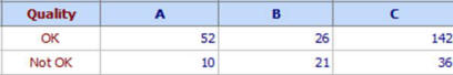
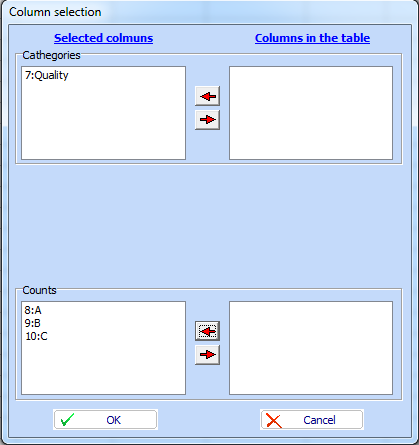
The first column (named in our example Quality) is defined as “Type”, the other columns are considered as “Data”.
The question is whether there are differences in the quality of supplies fulfillment? Statistically this problem can be solved by hypothesis testing. Define following hypotheses:
Null hypothesis: Classifications across rows and columns are independent
Alternative hypothesis: Classifications across rows and columns are not independent
Following notations will be used:
•The procedure is as follows:
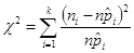
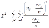
1. Calculate:
Null hypothesis is accepted
if ,
where  .
.
QstatLab calculates a probability Р. The null hypothesis is accepted if P > 0.05 and if Р < 0.05 the null hypothesis is rejected.
This algorithm works well enough
if the estimated number of events in each cell  is larger than 5.
Example with QstatLab:
The program can be activated as follows:
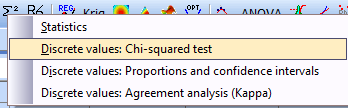
Click „Discrete values:Chi squared test” and select columns as follows:
Click „OK“and following solution will be obtained:
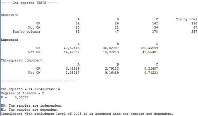
As P < 0.05 we conclude that the factor “Supplier” is significant, i.e. the results depend on the supplier. Chi-squared component can show how big the difference between the results of different suppliers is. The largest component is for supplier B. For this supplier the differences between the expected and the observed values of supplies with quality OK and NOK is largest. Twenty six supplies of quality OK are observed, while the expected supplies of quality OK are 36. Also 21 supplies of quality NOK are observed, while the expected ones are 11.
The number of categories (factor levels) for each factor can be any one as is shown in the example that follows.
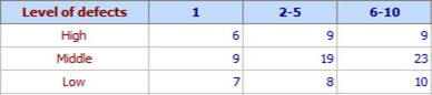
Example 2. One of the criteria for workers’ assessment in a factory is the number of defectives in 1000 produced parts. The work is monotonous and it is expected that after the initial training period the human motivation will go down. Considered are 100 workers divided into 3 categories: Category A – workers having up to 1 year experience, category B – workers with working experience between 2 to 5 years and category C - workers with experience from 6 to 10 years. The level of defects is divided into 3 categories: high, middle and low. We want to understand if the level of defects depends on working experience (file: Contingency.qsl).
The program can be activated as shown in Example 1. Following results are obtained:
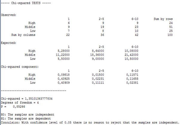
As P > 0.05 it is accepted that the factor “Experience” is insignificant. The level of defects does not depend on workers’ experience.