Airfoil shape optimization

File: airfoil.qsl

 

Use the Airfoil.exe application to familiarize yourself with the problem:

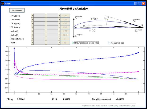
Vary the airfoil shape control parameters (using the slide buttons) and observe their effect on the lift (Clift), drag (CDrag) and pitching moment (Cm). The aim of this tutorial is to find a shape that maximizes lift, minimizes drag and pitching moment. What is the best solution you could find manually? Record your findings.

 

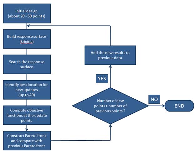
Now let’s see if we can improve this design by using computational procedures. The following flowchart represent the logic and sequence of activities.

1.   Open file airfoil.qsl

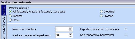
2.   Build an initial design of experiments consisting of 30 designs. As we will be using kriging later, it is recommended that the designs are uniformly distributed using an Lptau algorithm. Use the DOE icon  , select LPTau and enter 30 for the Maximum number of experiments:

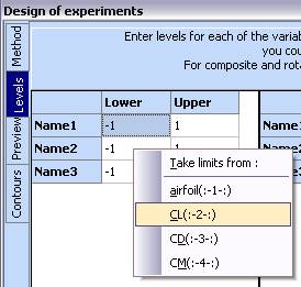
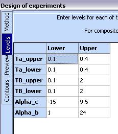
3.   Go to the ‘Levels’ tab and do a right-click in the first table. Choose CL(:-2-:). This will take the correct lower and upper boundaries for the variables

 

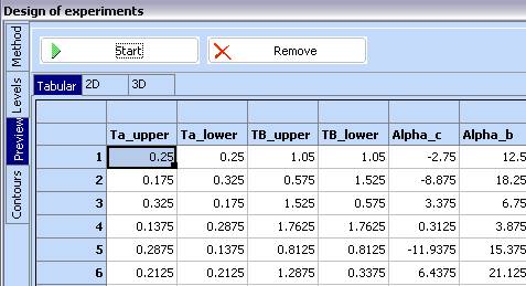
4.   Change to the Preview tab and click ‘Generate’ to obtain the design. Then use the  button to transfer it to the spreadsheet.

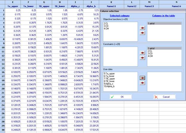
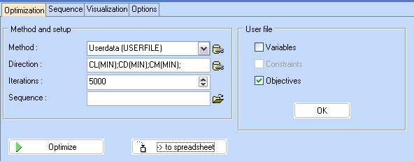
5.   Compute the values of CL, CD and CM for these designs. Use the Optimization tool:

 

 

6.   Once the optimization completes, transfer the values of the objectives back to the spreadsheet, using the ‘-> to spreadsheet’ button:

 

7.   Use the Kriging tool to construct a Krige model for the first objective function - CL

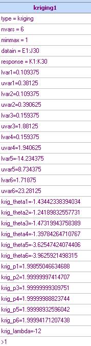
8.   Use ‘Calculate’ or ‘Start tuning’ to initiate the hyper-parameters computations. By default 4 cycles will be carried out and the best CLF of all 4 cycles will be used. At the end of the tuning a brief analysis of the model is shown. The meaning of the columns is as follows:

Observed – the experimental data

Predicted – the value computed by the model

Residual = Observed – Predicted

Error – the mean squared error

Exp. Improvement – the value of the expected improvement

Total residual - Sum of squares of the residuals

Total error - Sum of the mean squared errors

Note that the predictions and errors at each design point are computed after taking this design point out of the data available during predictions. Total residual 0.000158223869045627

 

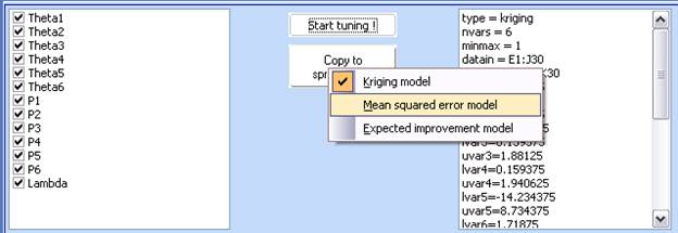
9.   Three models are available – prediction, MSE (mean squared error), and EI (expected improvement). Copy all of them to the spreadsheet. Use the Copy to spreadsheet button. To select which model to copy, right click on the same button and then click the button again to actually transfer to the spreadsheet:

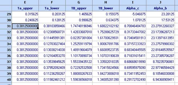
10.  The three models should appear in the spreadsheet:

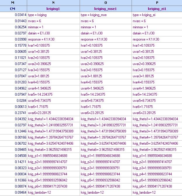
Kriging1 – prediction model for CL;

Kriging_mse1 – mean squared error for CL;

Kriging_ei1 – expected improvement mode for CL;

 

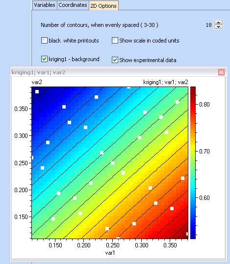
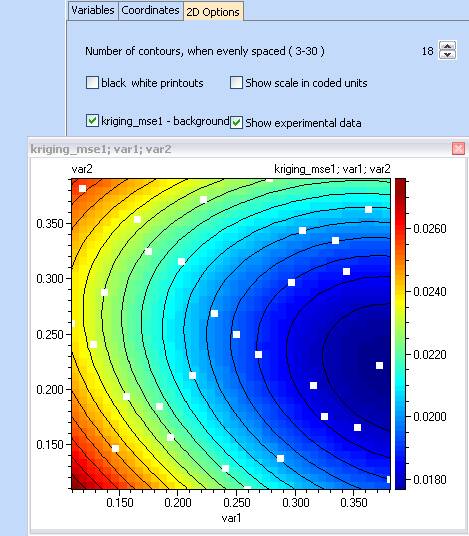
11.  We can now plot some of the three models.

 

 

12.  Repeat steps 7-11 to obtain models for CD and CM

13.  You should now have the following models in the table:

Kriging1 – prediction model for CL;

Kriging_mse1 – mean squared error for CL;

Kriging_ei1 – expected improvement mode for CL;

Kriging2 – prediction model for CD;

Kriging_mse2 – mean squared error for CD;

Kriging_ei2 – expected improvement mode for CD;

Kriging3 – prediction model for CM;

Kriging_mse3 – mean squared error for CM;

Kriging_ei3 – expected improvement mode for CM;

 

14.  Optimization. We would now like to find what is the optimal airfoil shape that will maximize lift (and keep it above 1), reduce drag and pitching moment. The optimization could be run directly on the VGK model, but this might be time and resource ineffective. The optimization task can be defined as follows:

Max(Kriging1); Min(Kriging2); Min(kriging3); and Kriging1 > 1

15.  Therefore add ‘>1’ at the end of the kriging1 model:

 

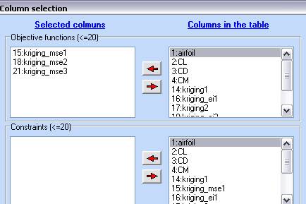
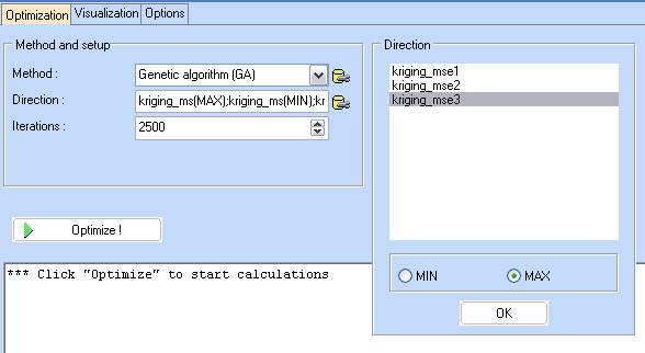
16.  Use the optimization tool to carry out multiobjective optimization:

 

 

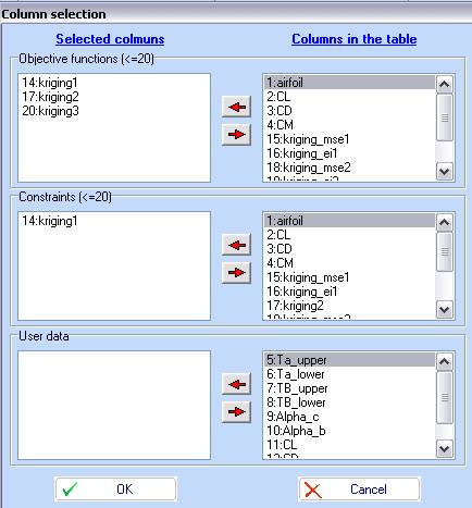
17.  Select MAX for the first objective function:

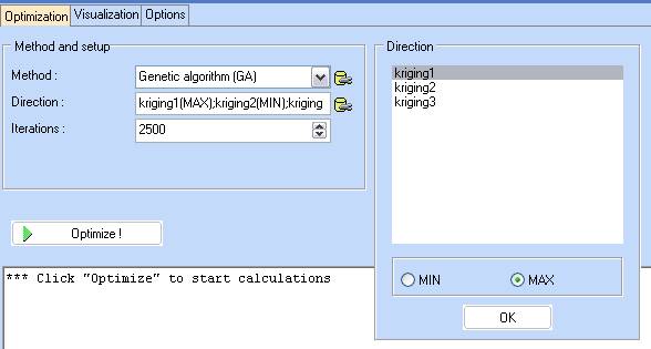
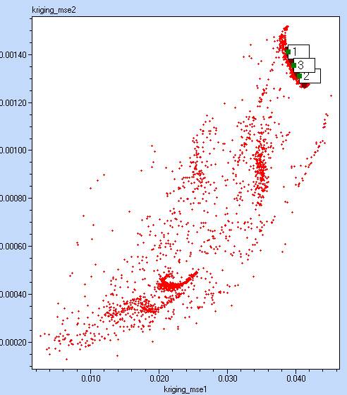
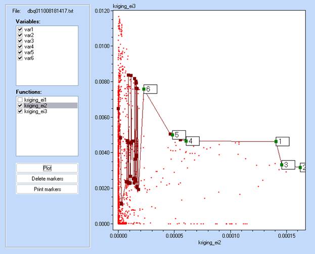
18.  Click ’Optimize!’ and after completion, go to the Visualization tab to inspect the Pareto front

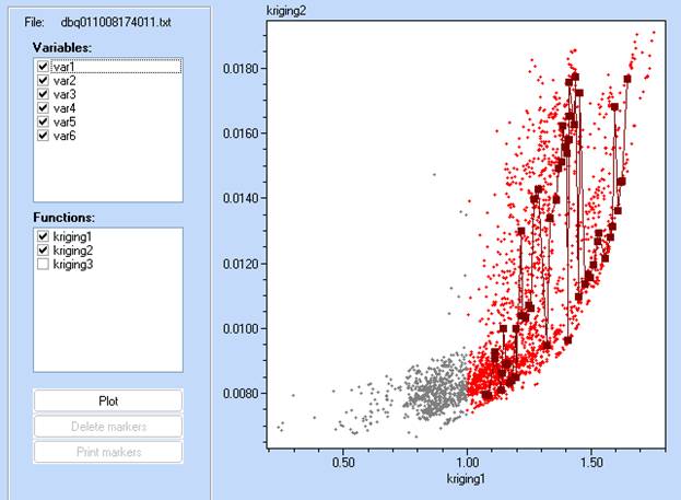
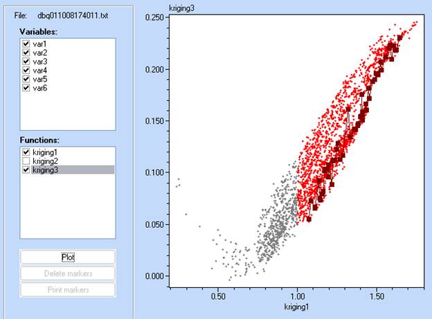
19.  In each of the projections we can now mark several best points and observe where they appear in the other projection.

 

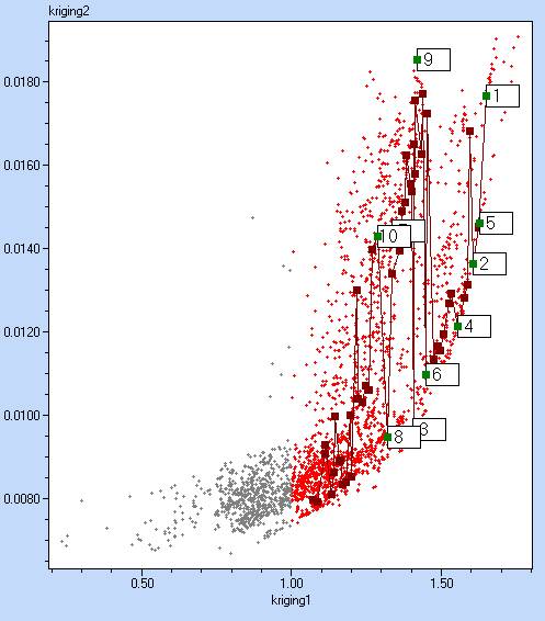
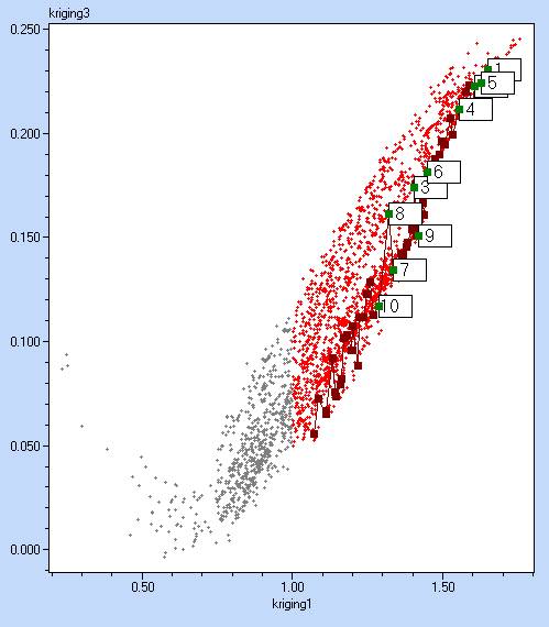
One can see that for instance marker 10 appears to be a good solution for kriging1/kriging3, it is a bad one for kriging1/kriging2. These results could be further discussed and tested against other engineering considerations. Values associated with each marker can be seen in the Optimization tab.

These results were obtained using a prediction that might not be accurate. That is why we should now select points to for updates. There are several strategies for update selection:

• Designs that belong to the predicted pareto front (kriging 1,2,3)
• Designs which maximize the mean squared error (kriging_mse1,2,3)
• Designs which maximize the expected improvement (kriging_ei1,2,3).

 

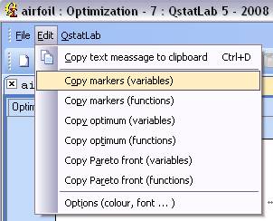
As we have just marked 10 points that belong to the predicted pareto front we can use them and add them to the table.

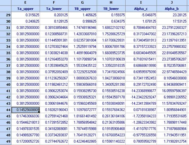
20.  Copy the values of the variables for each marker:

21.  And now paste them below the initial 30 designs:

22.  Build a pareto front of the maximums of the 3 MSE models. Use multiobjective optimization, and choose MAX for all three models:

 

 

23.  Click optimization and after completion – visualize. Mark several points:

 

24.  Copy and paste as shown in steps 20, 21

25.  Construct pareto front of the maximum expected improvements and mark several points. Note that the kriging_ei1 is always 0.

 

 

26.  Copy and paste as in steps 20, 21

 

 

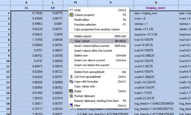
27.  We have now selected 19 updates in total that need to be evaluated. Clear all columns including those that contain the kriging models, but leave those that define the models and the variables. Clear – but not delete

 

 

28.  Compute the values of the three objectives as in steps 5 and 6, so that their values appear in columns K, L, M.

 

 

 

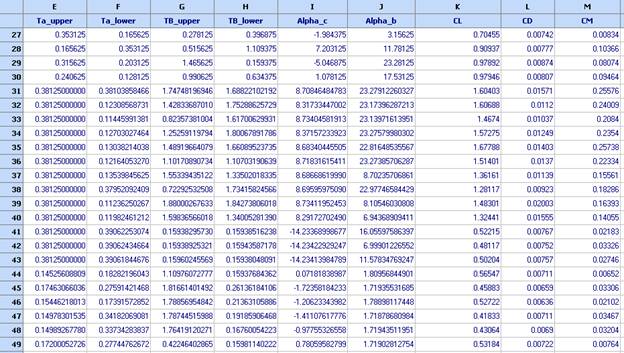
29.  Repeat from step 7. This will give us new kriging models based on the new updates. Note that for CL the residual error has now dropped to Total residual 1.09062107702609E-15.

30.  Note that the tuning of the krigs has become slower, which is due to the increased number of observations. QstatLab can choose the best 50 points to restrict the infinite increase of the data used for training.

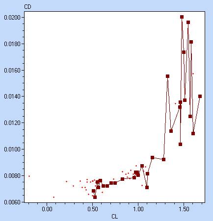
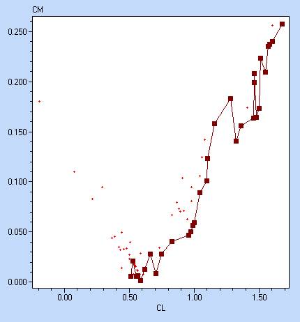
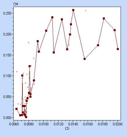
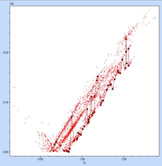
31.  After 3 updates, we have accumulated 72 experimental points, plotted below. It is seen that very few runs do not belong to the pareto front, which shows that the procedure was effective.

 

 

 

 

Comparison

 

Solutions after 2500 direct runs                              Solution after 75 runs with RSM

 

A comparison between direct optimization and optimization using RSM clearly shows the advantage in using RSMs